Tutorial: Working with Nodal Attributes in Network Models
Day 3 | Network Modeling for Epidemics
This tutorial will show how to estimate a dynamic network model for a two-group network: instead of one large group of homogeneous nodes, now we’ll have two groups that can differ based on their behavior or biology. Here, we will motivate this with a heterosexual network in which the groups may represent females and males in the population.
To get started, load the EpiModel library.
library(EpiModel)We also recommend that you clear your environment to avoid any leftover objects from the last tutorials or labs.
rm(list = ls())For this particular tutorial, we will set the seed to ensure reproducible results.
set.seed(12345)Network Model
For the network model parameterization, we will review how to fit a two-group model with a differential degree distribution by group.
Initialization
The number in each group will be 250 nodes.
num.g1 <- num.g2 <- 250
nw <- network_initialize(n = num.g1 + num.g2)
nw
Network attributes:
vertices = 500
directed = FALSE
hyper = FALSE
loops = FALSE
multiple = FALSE
bipartite = FALSE
total edges= 0
missing edges= 0
non-missing edges= 0
Vertex attribute names:
vertex.names
No edge attributesWe use the following function to define a nodal attribute,
group, and then set it on the network. We can print out the
network again to see that it has been added to the list of vertex
attributes. To use group as a special attribute (see
paragraph below), the values of group must be
1 and 2 only.
group <- rep(1:2, times = c(num.g1, num.g2))
nw <- set_vertex_attribute(nw, attrname = "group", value = group)
nw
Network attributes:
vertices = 500
directed = FALSE
hyper = FALSE
loops = FALSE
multiple = FALSE
bipartite = FALSE
total edges= 0
missing edges= 0
non-missing edges= 0
Vertex attribute names:
group vertex.names
No edge attributesWe can use get_vertex_attribute to extract the same
attribute from the network object:
get_vertex_attribute(nw, "group") [1] 1 1 1 1 1 1 1 1 1 1 1 1 1 1 1 1 1 1 1 1 1 1 1 1 1 1 1 1 1 1 1 1 1 1 1 1 1
[38] 1 1 1 1 1 1 1 1 1 1 1 1 1 1 1 1 1 1 1 1 1 1 1 1 1 1 1 1 1 1 1 1 1 1 1 1 1
[75] 1 1 1 1 1 1 1 1 1 1 1 1 1 1 1 1 1 1 1 1 1 1 1 1 1 1 1 1 1 1 1 1 1 1 1 1 1
[112] 1 1 1 1 1 1 1 1 1 1 1 1 1 1 1 1 1 1 1 1 1 1 1 1 1 1 1 1 1 1 1 1 1 1 1 1 1
[149] 1 1 1 1 1 1 1 1 1 1 1 1 1 1 1 1 1 1 1 1 1 1 1 1 1 1 1 1 1 1 1 1 1 1 1 1 1
[186] 1 1 1 1 1 1 1 1 1 1 1 1 1 1 1 1 1 1 1 1 1 1 1 1 1 1 1 1 1 1 1 1 1 1 1 1 1
[223] 1 1 1 1 1 1 1 1 1 1 1 1 1 1 1 1 1 1 1 1 1 1 1 1 1 1 1 1 2 2 2 2 2 2 2 2 2
[260] 2 2 2 2 2 2 2 2 2 2 2 2 2 2 2 2 2 2 2 2 2 2 2 2 2 2 2 2 2 2 2 2 2 2 2 2 2
[297] 2 2 2 2 2 2 2 2 2 2 2 2 2 2 2 2 2 2 2 2 2 2 2 2 2 2 2 2 2 2 2 2 2 2 2 2 2
[334] 2 2 2 2 2 2 2 2 2 2 2 2 2 2 2 2 2 2 2 2 2 2 2 2 2 2 2 2 2 2 2 2 2 2 2 2 2
[371] 2 2 2 2 2 2 2 2 2 2 2 2 2 2 2 2 2 2 2 2 2 2 2 2 2 2 2 2 2 2 2 2 2 2 2 2 2
[408] 2 2 2 2 2 2 2 2 2 2 2 2 2 2 2 2 2 2 2 2 2 2 2 2 2 2 2 2 2 2 2 2 2 2 2 2 2
[445] 2 2 2 2 2 2 2 2 2 2 2 2 2 2 2 2 2 2 2 2 2 2 2 2 2 2 2 2 2 2 2 2 2 2 2 2 2
[482] 2 2 2 2 2 2 2 2 2 2 2 2 2 2 2 2 2 2 2In core EpiModel, the group attribute has a
special role for these built-in models that we are exploring in this
course. We can, and will, use other nodal attributes on the
network to model elements like age or race within the network structure.
But group is special because it allows for easy
parameterization of heterogeneous epidemic parameters (e.g.,
group-specific recovery rates). Epidemic parameters stratified by other
attributes can also be arbitrarily added, but this requires some
additional programming of the epidemic modules in EpiModel. We’ll get to
that at the end of Day 4 and spend most of Day 5 on this.
Degree Distributions
Next, the group-specific degree distributions are specified as the fractions of each group that have 0, 1, 2, and 3 or more edges at any one time (momentary degree). Within this two-group framework, the first group will represent women and the second men. In our hypothetical empirical data, women exhibit less concurrency than men, but also fewer isolates. The following are those fractional distributions.
deg.dist.g1 <- c(0.40, 0.55, 0.04, 0.01)
deg.dist.g2 <- c(0.54, 0.31, 0.10, 0.05)
In our model, we will use a mean degree of 0.66. How do our degree
distributions compare to the distribution expected under a Poisson
probability mass function with a rate equal to this the mean degree? The
dpois function in R returns the probability mass for degree
0 through 2 and ppois sums the cumulative mass for degree
3+.
pois.dists <- c(dpois(0:2, lambda = 0.66),
                ppois(2, lambda = 0.66, lower.tail = FALSE))
This barplot compares the two observed and the one estimated fractional degree distribution, each adding to 100%. The degree distribution for men more closely matches that of the Poisson distribution, but still has slightly less concurrency than expected.
par(mar = c(3,3,2,1), mgp = c(2,1,0), mfrow = c(1,1))
barplot(cbind(deg.dist.g1, deg.dist.g2, pois.dists),
        beside = TRUE, ylim = c(0, 0.6), col = 1:4)
legend("topright", legend = paste0("deg", 0:3),
       pch = 15, col = 1:4,
       cex = 0.9, bg = "white")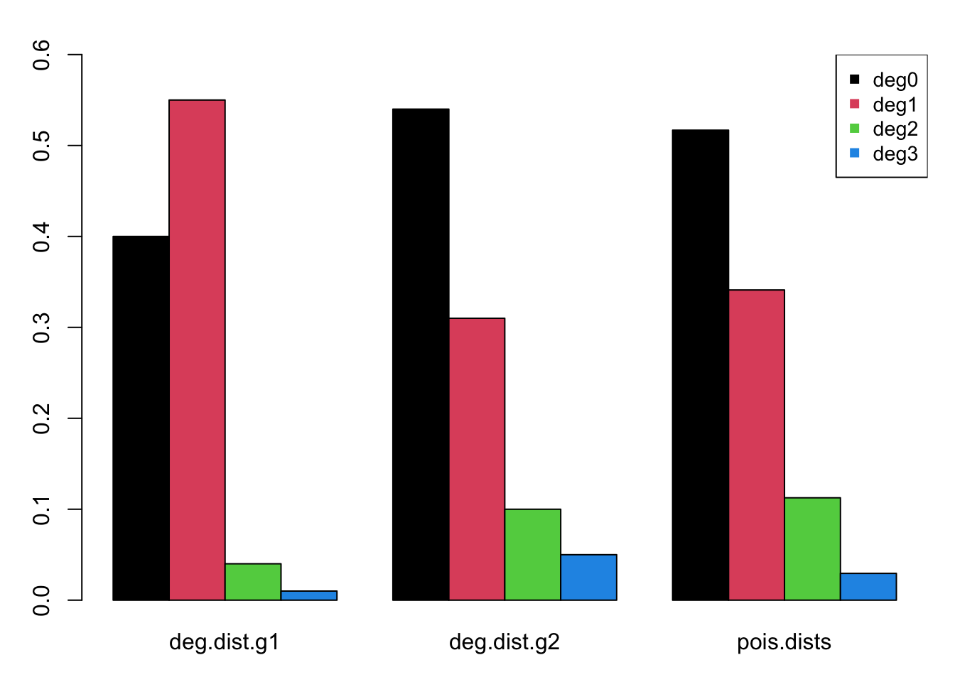
In this model, we will represent a multi-group network in which there
is purely disortative mixing (by sex) to represent heterosexual contact.
With this parameterization, and either a differential group size or
degree distribution, the overall number of edges expected from
each group must match. The EpiModel function
check_degdist_bal takes as input two group sizes and two
fractional degree distributions and checks whether the total number of
implied edges is the same. Note that this constraint of matching
edges is relaxed when mixing is not purely disortative (because some
edges occur within group); nonetheless, TERGM parameterization still
does require a single edges statistic.
check_degdist_bal(num.g1, num.g2,
                  deg.dist.g1, deg.dist.g2)
Degree Distribution Check
=============================================
g1.dist g1.cnt g2.dist g2.cnt
Deg0 0.40 100.0 0.54 135.0
Deg1 0.55 137.5 0.31 77.5
Deg2 0.04 10.0 0.10 25.0
Deg3 0.01 2.5 0.05 12.5
Edges 1.00 165.0 1.00 165.0
=============================================
** Edges balanced ** Formation and Dissolution
Since we have not specified any nodal attributes for the network
other than group, the formation model will only consider aspects of the
group-specific degree distribution and mixing on group. ERGM model term
degree allows for stratification by a nodal attribute. The
0:1 notation within a single degree term below is a
short-hand way of writing multiple degree terms (e.g.,
degree(0) + degree(1)). The nodematch term is
a may to represent the edges on a diagonal of a mixing matrix for the
specified attribute (i.e., within group mixing).
formation <- ~edges + degree(0:1, by = "group") + nodematch("group")For the target statistics, we specify the number of edges as a
function of mean degree as 0.66 (500/2 * 0.66 = 165). Or we
can input the numbers directly from the check_degdist_bal
output, where the Edges indicates the edges and the
g1.cnt the numbers of group 1 nodes with degree 0 to 3, and
g2.cnt the same for group 2 nodes. There are four target
statistics needed for the degree terms: 2 for each degree term times 2
for each group. They are input by group and then by degree (so degree 0
for group 1, then degree 1 for group 1, then degree 0 for group 2, and
degree 1 for group 2). In this particular model, we will not overfit by
including all possible degree terms (i.e., a count of persons with
degrees 2 and 3). Finally, the target statistic for nodematch with a
purely disortative mixing model is 0: there are no edges between persons
matched on the value of the group variable.
target.stats <- c(165, 100, 137.5, 135, 77.5, 0)To recap the formulation of the target statistics:
edgesis a count of edgesdegreeis a count of nodes (whith a particular degree)nodematchis a count of edges (matched on a nodal attribute)
The dissolution model is parameterized the same as the prior example but with a shorter partnership duration than the first tutorial.
coef.diss <- dissolution_coefs(dissolution = ~offset(edges), duration = 10)
coef.diss
Dissolution Coefficients
=======================
Dissolution Model: ~offset(edges)
Target Statistics: 10
Crude Coefficient: 2.197225
Mortality/Exit Rate: 0
Adjusted Coefficient: 2.197225Estimation
The netest function is used for network model
fitting.
est <- netest(nw, formation, target.stats, coef.diss)For the dynamic diagnostics, we simulate from the model fit. The edges have a small bias, due to the relatively short duration. It is important to consider both the relative and absolute magnitude of the bias here. For our purposes, this fit is good enough to move forward!
dx <- netdx(est, nsims = 10, nsteps = 500, ncores = 5,
            nwstats.formula = ~edges + degree(0:3, by = "group"))
Network Diagnostics
-----------------------
- Simulating 10 networks
- Calculating formation statistics
- Calculating duration statistics
- Calculating dissolution statistics
dxEpiModel Network Diagnostics
=======================
Diagnostic Method: Dynamic
Simulations: 10
Time Steps per Sim: 500
Formation Diagnostics
-----------------------
Target Sim Mean Pct Diff Sim SD
edges 165.0 158.569 -3.897 10.219
deg0.group1 100.0 106.681 6.681 8.179
deg1.group1 137.5 130.553 -5.052 8.028
deg2.group1 NA 10.585 NA 3.103
deg3.group1 NA 1.904 NA 1.403
deg0.group2 135.0 138.623 2.684 6.669
deg1.group2 77.5 75.903 -2.060 7.155
deg2.group2 NA 26.018 NA 4.460
deg3.group2 NA 7.548 NA 2.549
nodematch.group 0.0 NA NA NA
Duration Diagnostics
-----------------------
Target Sim Mean Pct Diff Sim SD
edges 10 9.974 -0.261 0.15
Dissolution Diagnostics
-----------------------
Target Sim Mean Pct Diff Sim SD
edges 0.1 0.101 0.625 0.001This is confirmed when we plot the diagnostics.
plot(dx)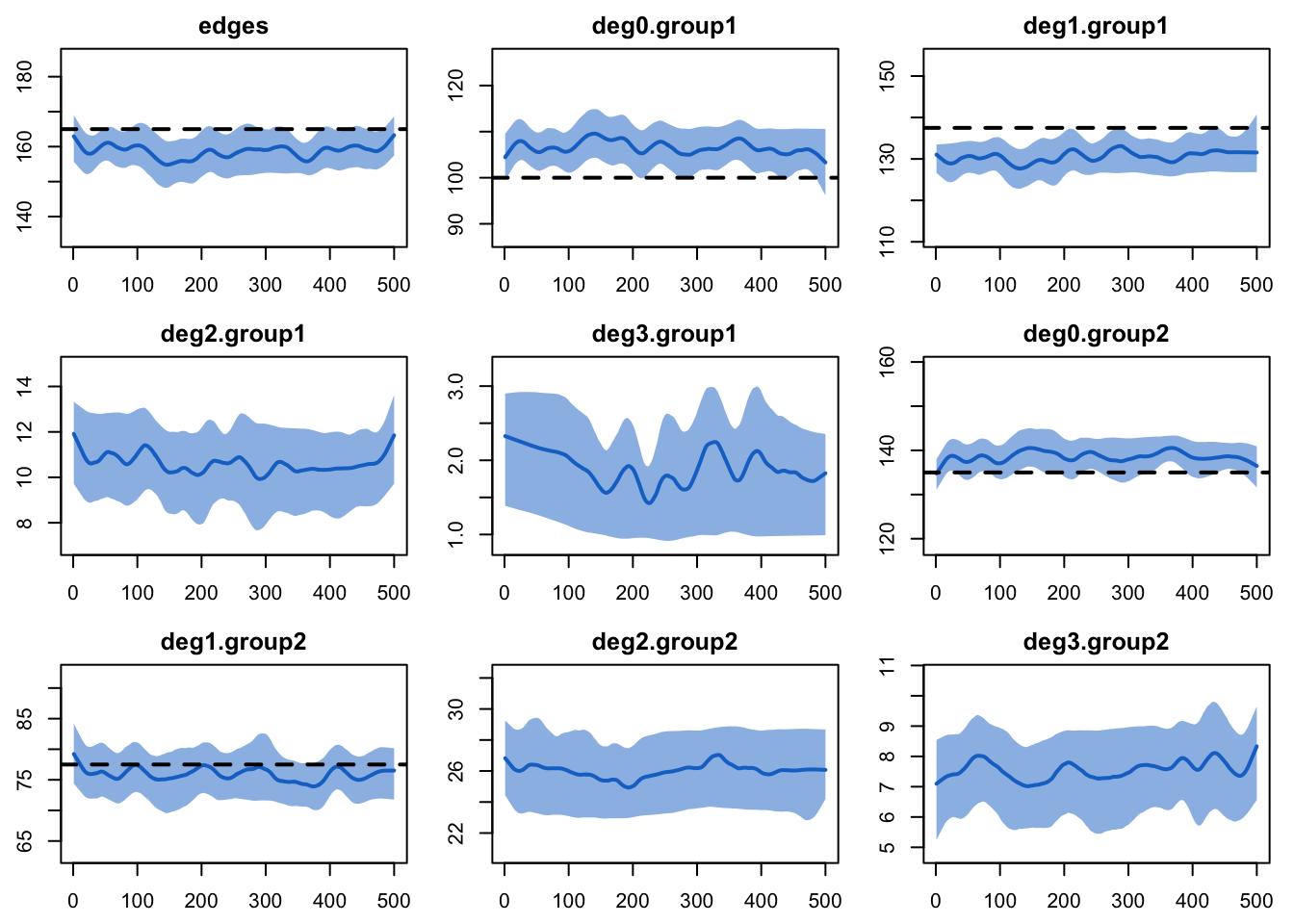
To compare simulations against out-of-model predictions, let’s look again at the expected degree 2 and degree 3 for each group. The simulation means are pretty close to those expectations.
check_degdist_bal(num.g1, num.g2,
                  deg.dist.g1, deg.dist.g2)
Degree Distribution Check
=============================================
g1.dist g1.cnt g2.dist g2.cnt
Deg0 0.40 100.0 0.54 135.0
Deg1 0.55 137.5 0.31 77.5
Deg2 0.04 10.0 0.10 25.0
Deg3 0.01 2.5 0.05 12.5
Edges 1.00 165.0 1.00 165.0
=============================================
** Edges balanced ** Epidemic Model
For the disease simulation, we will simulate an SIR epidemic in a closed population.
Parameterization
The epidemic model parameters are below. In this tutorial, we will use biological parameters for the infection probability per act and recovery rates as equal to demonstrate the impact of group-specific degree distributions on outcomes. Note that the group-specific parameters for the infection probability govern the risk of infection to persons in that mode given contact with persons in the other group.
param <- param.net(inf.prob = 0.2, inf.prob.g2 = 0.2,
                   rec.rate = 0.02, rec.rate.g2 = 0.02)
At the outset, 10 people in each group will be infected. For an SIR epidemic simulation, it is necessary to specify the number recovered in each group, here starting at 0.
init <- init.net(i.num = 10, i.num.g2 = 10,
                 r.num = 0, r.num.g2 = 0)
For control settings, we will simulate 5 epidemics over 500 time steps each. Here we use the multi-core functionality in our controls.
control <- control.net(type = "SIR", nsims = 5, nsteps = 500, ncores = 5)Simulation
The model is simulated by inputting the fitted network model, the epidemic parameters, the initial conditions, and control settings.
sim <- netsim(est, param, init, control)Printing the model object shows the inputs and outputs from the
simulation object. In particular, take note of the Variables listing;
the epidemic outputs for Group 1 are listed without a suffix whereas the
outputs for Group 2 are listed with a .g2 suffix.
simEpiModel Simulation
=======================
Model class: netsim
Simulation Summary
-----------------------
Model type: SIR
No. simulations: 5
No. time steps: 500
No. NW groups: 2
Fixed Parameters
---------------------------
inf.prob = 0.2
rec.rate = 0.02
inf.prob.g2 = 0.2
rec.rate.g2 = 0.02
act.rate = 1
groups = 2
Model Output
-----------------------
Variables: s.num i.num r.num num s.num.g2 i.num.g2
r.num.g2 num.g2 si.flow si.flow.g2 ir.flow ir.flow.g2
Networks: sim1 ... sim5
Transmissions: sim1 ... sim5
Formation Diagnostics
-----------------------
Target Sim Mean Pct Diff Sim SD
edges 165.0 159.873 -3.107 9.304
deg0.group1 100.0 105.824 5.824 7.765
deg1.group1 137.5 131.188 -4.591 8.041
deg0.group2 135.0 138.385 2.507 6.386
deg1.group2 77.5 75.462 -2.630 7.284
nodematch.group 0.0 0.000 NaN 0.000
Dissolution Diagnostics
-----------------------
Target Sim Mean Pct Diff Sim SD
edges 0.1 NaN NaN NANote also that the print output includes the names of the individual
modules. For these two-group models, EpiModel automatically selects
which modules and functions to use. For extension modules (that do not
have have a type input), you will need to specify this.
Analysis
Similar to the first tutorial, plotting the netsim
object shows the prevalence for each disease state in the model over
time.
par(mfrow = c(1, 1))
plot(sim, main = "Disease State Sizes")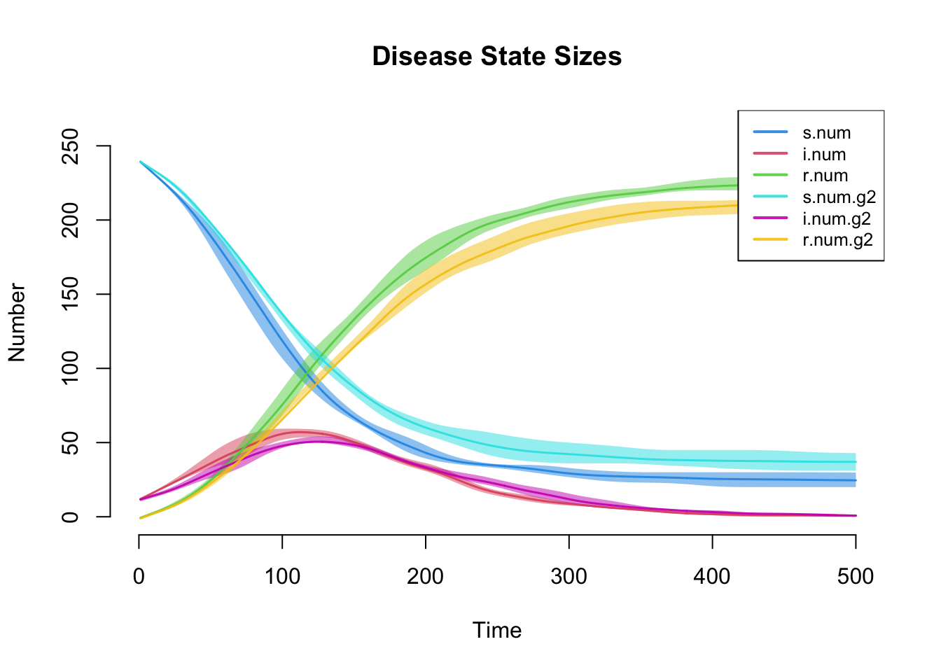
This plot more clearly shows prevalence and incidence by mode. Interestingly, women (Group 1) have a slightly higher prevalence of disease during the main epidemic period, and more women than men end up in the recovered state. Men and women have the same mean degree but men have a higher prevalence of concurrency (degree 2+) than women. Following epidemiological and network theory, conditional on mean degree (which is the same for both groups in this model), concurrency increases the risk of transmission but not acquisition. So therefore, women bear the higher burden of male concurrency. Your course instructor, Steve Goodreau, has prepared an excellent tutorial and exercise set on this topic.
par(mfrow = c(1,2))
plot(sim, y = c("i.num", "i.num.g2"), popfrac = TRUE,
     qnts = FALSE, ylim = c(0, 0.4), legend = TRUE)
plot(sim, y = c("si.flow", "si.flow.g2"),
     qnts = FALSE, ylim = c(0, 2.5), legend = TRUE)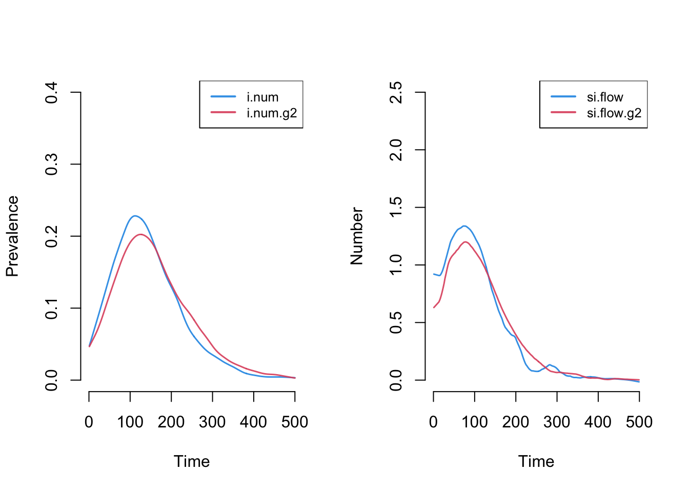
It is possible to plot the color-coded static network at various time points during the simulation, as in the last tutorial. This helps to visualize how womens’ (circle) risk is dependent on their male (square) partners’ network connections.
par(mfrow = c(1, 1), mar = c(0, 0, 0, 0))
plot(sim, type = "network", col.status = TRUE, at = 50,
     sims = "mean", shp.g2 = "square")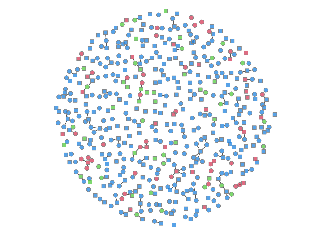
It is possible to add new variables to an existing model object with
mutate_epi, which takes inspiration from the
mutate functions in the tidyverse. With a time
step unit of a week, we can calculate standardized incidence rates per
100 person-years at risk using the following approach. The
mutate_epi function takes a netsim object and
adds a new variable.
sim <- mutate_epi(sim, ir.g1 = (si.flow / s.num) * 100 * 52,
                       ir.g2 = (si.flow.g2 / s.num.g2) * 100 * 52)
Printing out the object, you can see that these two new variables are in the variable list.
simEpiModel Simulation
=======================
Model class: netsim
Simulation Summary
-----------------------
Model type: SIR
No. simulations: 5
No. time steps: 500
No. NW groups: 2
Fixed Parameters
---------------------------
inf.prob = 0.2
rec.rate = 0.02
inf.prob.g2 = 0.2
rec.rate.g2 = 0.02
act.rate = 1
groups = 2
Model Output
-----------------------
Variables: s.num i.num r.num num s.num.g2 i.num.g2
r.num.g2 num.g2 si.flow si.flow.g2 ir.flow ir.flow.g2 ir.g1
ir.g2
Networks: sim1 ... sim5
Transmissions: sim1 ... sim5
Formation Diagnostics
-----------------------
Target Sim Mean Pct Diff Sim SD
edges 165.0 159.873 -3.107 9.304
deg0.group1 100.0 105.824 5.824 7.765
deg1.group1 137.5 131.188 -4.591 8.041
deg0.group2 135.0 138.385 2.507 6.386
deg1.group2 77.5 75.462 -2.630 7.284
nodematch.group 0.0 0.000 NaN 0.000
Dissolution Diagnostics
-----------------------
Target Sim Mean Pct Diff Sim SD
edges 0.1 NaN NaN NAAfter we add the new variable, we can plot and analyze it like any other built-in variable.
par(mar = c(3,3,2,1))
plot(sim, y = c("ir.g1", "ir.g2"), legend = TRUE,
     main = "Standardized Incidence Rates by Group")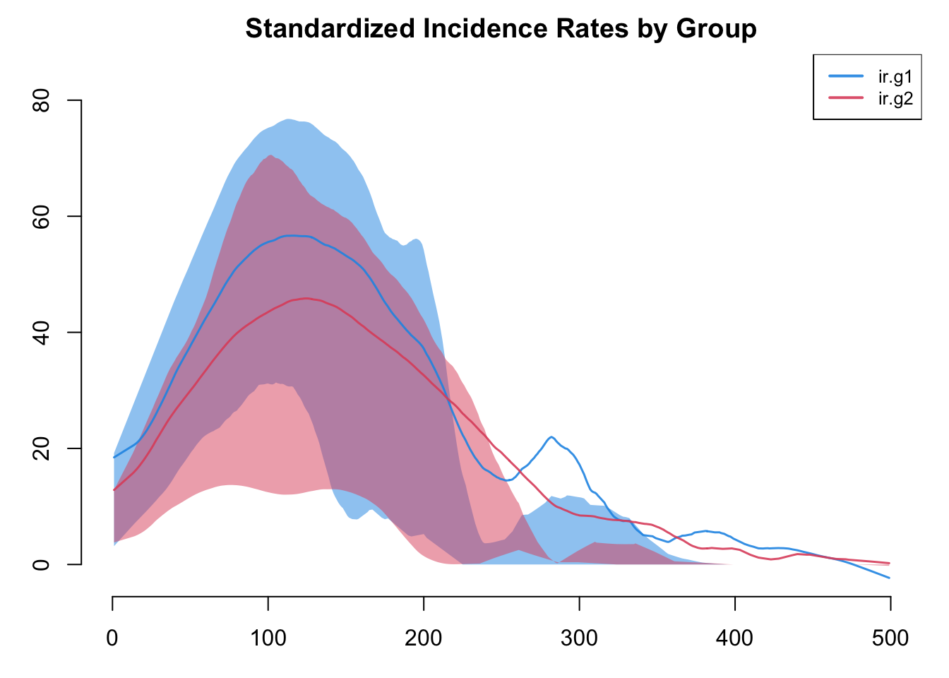
Incidence rates in particular are often highly variable. The plot by default will use a loess smoother so some of this variability may be lost. Therefore, it is worth inspecting the non-smoothed plots too.
plot(sim, y = c("ir.g1", "ir.g2"), legend = TRUE,
     mean.smooth = FALSE, qnts = FALSE, mean.lwd = 1,
     main = "Standardized Incidence Rates by Group (Non-Smoothed)")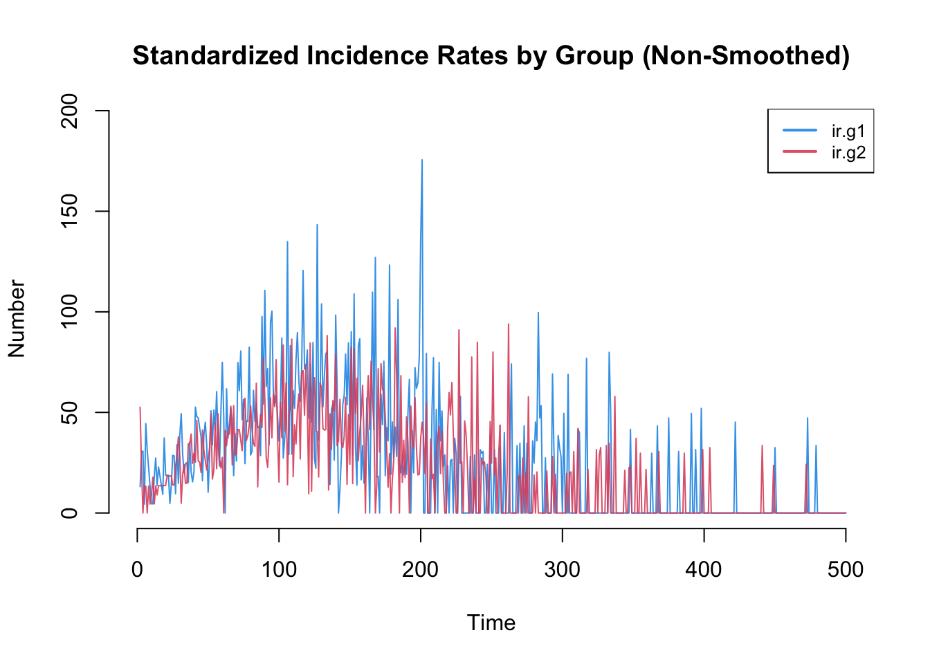
As another exercise, let’s extract the data into a data frame and
then calculate some other relevant summary statistics. By default
as.data.frame will extract the individual simulation data
in each row, but by specifying out = "mean" we can see the
time specific averages for all the variables across simulations. The
variables in this data frame include both the original variables from
netsim plus the two new ones we added with
mutate_epi.
df <- as.data.frame(sim, out = "mean")
head(df, 10)
time s.num i.num r.num num s.num.g2 i.num.g2 r.num.g2 num.g2 si.flow
1 1 240.0 10.0 0.0 250 240.0 10.0 0.0 250 NaN
2 2 239.4 10.6 0.0 250 237.6 12.2 0.2 250 0.6
3 3 238.0 12.0 0.0 250 236.6 13.2 0.2 250 1.4
4 4 236.6 13.2 0.2 250 236.6 13.2 0.2 250 1.4
5 5 236.4 13.4 0.2 250 236.0 13.6 0.4 250 0.2
6 6 234.4 15.4 0.2 250 235.4 13.6 1.0 250 2.0
7 7 233.0 16.6 0.4 250 235.4 13.2 1.4 250 1.4
8 8 232.0 16.6 1.4 250 234.8 13.8 1.4 250 1.0
9 9 231.4 16.2 2.4 250 234.6 14.0 1.4 250 0.6
10 10 231.2 15.2 3.6 250 234.2 14.2 1.6 250 0.2
si.flow.g2 ir.flow ir.flow.g2 ir.g1 ir.g2
1 NaN NaN NaN NaN NaN
2 2.4 0.0 0.2 13.090960 52.622132
3 1.0 0.0 0.0 30.680578 21.996710
4 0.0 0.2 0.0 30.754488 0.000000
5 0.6 0.0 0.2 4.406780 13.257843
6 0.6 0.0 0.6 44.445092 13.314421
7 0.0 0.2 0.4 31.322084 0.000000
8 0.6 1.0 0.0 22.510823 13.390558
9 0.2 1.0 0.0 13.468348 4.444444
10 0.4 1.2 0.2 4.521739 8.832312One interesting summary statistic for an SIR epidemic is the
cumulative incidence. Here are the mean cumulative incidences in the
first and second groups across simulations. It is necessary here to use
na.rm = TRUE to calculate these statistics by removing the
first row where the value is undefined.
sum(df$si.flow, na.rm = TRUE)[1] 215.4sum(df$si.flow.g2, na.rm = TRUE)[1] 203Here are two more that may be of interest: the time point of the peak standardized incidence rates, and also the value of the incidence rate at that time point.
which.max(df$ir.g1)[1] 201df$ir.g1[which.max(df$ir.g1)][1] 175.588plot(sim, y = "ir.g1",
mean.smooth = FALSE, qnts = FALSE, mean.lwd = 1,
main = "Time and Value of Peak Incidence in Females (Group 1)")
points(which.max(df$ir.g1), df$ir.g1[which.max(df$ir.g1)], cex = 3)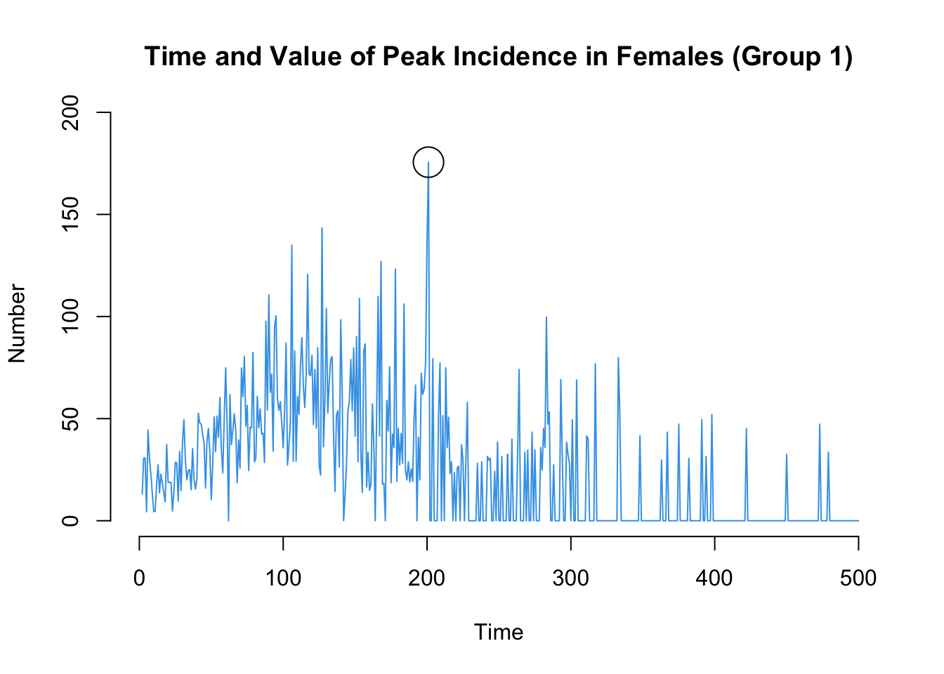
The transmission matrix again shows the individual transmission events that occurred at each time step, along with information about the infecting partner that may be relevant.
tm <- get_transmat(sim)
head(tm, 15)
at sus inf infDur transProb actRate finalProb
1 2 425 135 77 0.2 1 0.2
2 3 291 194 88 0.2 1 0.2
3 3 486 62 28 0.2 1 0.2
4 3 402 91 103 0.2 1 0.2
5 4 73 486 1 0.2 1 0.2
6 4 164 423 88 0.2 1 0.2
7 4 149 266 2 0.2 1 0.2
8 6 140 423 90 0.2 1 0.2
9 6 24 425 4 0.2 1 0.2
10 6 187 486 3 0.2 1 0.2
11 7 59 423 91 0.2 1 0.2
12 7 117 397 27 0.2 1 0.2
13 8 65 328 28 0.2 1 0.2
14 9 240 266 7 0.2 1 0.2
15 10 339 24 4 0.2 1 0.2The infDur column shows the duration of infection (in
time steps) of the infecting partner at the point of transmission. For
example, an event with an infDur of 1 means that the
infecting partner had just become infected themselves in the prior time
step. This is the proportion of transmission that occured in that
state.
mean(tm$infDur == 1)[1] 0.04941176One can also convert this into a phylogeny for easier visualization
of these transmission chains. First, we convert the transmission matrix
into a phylo class object that can then be further analyzed
and visualized with the ape package. In this transmission
matrix, there are multiple trees found because we seeded the infection
with 20 people as initial conditions.
tmPhylo <- as.phylo.transmat(tm)found multiple trees, returning a list of 15phylo objectsHere is a standard phylogram of the first four trees. Some initial seeds lead to many downstream infections whereas others do not. Is this a function of underlying contact networks of the seeded nodes, the biology or behavior of those nodes, or something else? This could all be tested!
par(mfrow = c(2, 2), mar = c(0, 0, 0, 0))
plot(tmPhylo[[1]], show.node.label = TRUE, root.edge = TRUE, cex = 0.5)
plot(tmPhylo[[2]], show.node.label = TRUE, root.edge = TRUE, cex = 0.5)
plot(tmPhylo[[3]], show.node.label = TRUE, root.edge = TRUE, cex = 0.5)
plot(tmPhylo[[4]], show.node.label = TRUE, root.edge = TRUE, cex = 0.5)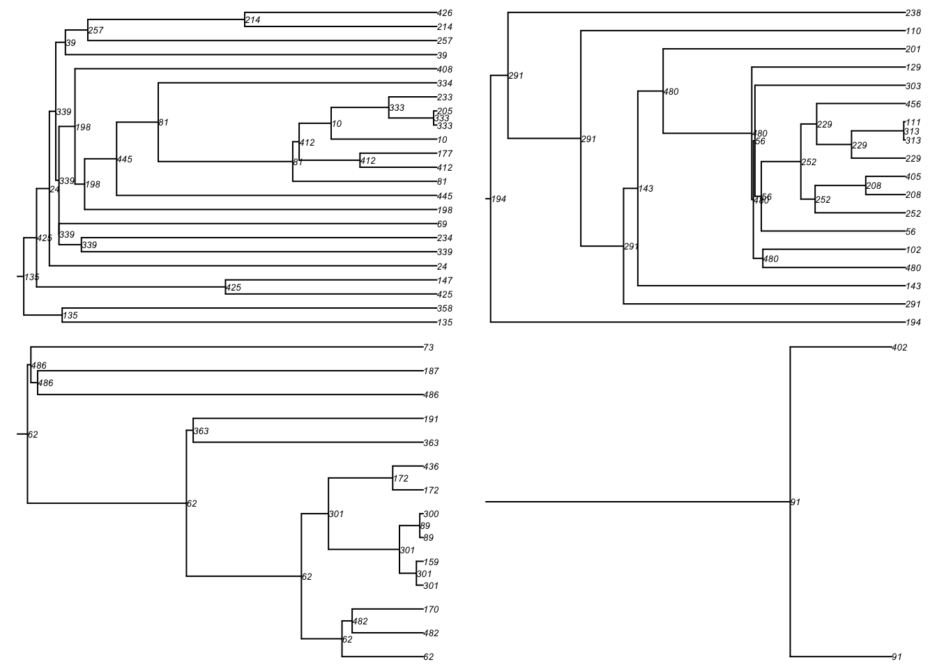
In phylo objects with multiple trees, each tree is
stored with a named object. Note that these names correspond to the ID
numbers in the transmission matrix itself. We can extract one tree like
so:
names(tmPhylo) [1] "seed_135" "seed_194" "seed_62" "seed_91" "seed_423" "seed_266"
[7] "seed_397" "seed_328" "seed_26" "seed_1" "seed_401" "seed_217"
[13] "seed_101" "seed_18" "seed_404"tmPhylo5 <- tmPhylo[[5]]Then we can plot that particular tree as a phylogram and other visual
types included in the ape package.
par(mfrow = c(2, 2), mar = c(0, 0, 0, 0))
plot(tmPhylo5, type = "phylogram",
     show.node.label = TRUE, root.edge = TRUE, cex = 0.5)
plot(tmPhylo5, type = "cladogram",
     show.node.label = TRUE, root.edge = TRUE, cex = 0.5)
plot(tmPhylo5, type = "fan",
     show.node.label = TRUE, root.edge = TRUE, cex = 0.5)
plot(tmPhylo5, type = "unrooted",
     show.node.label = TRUE, root.edge = TRUE, cex = 0.5)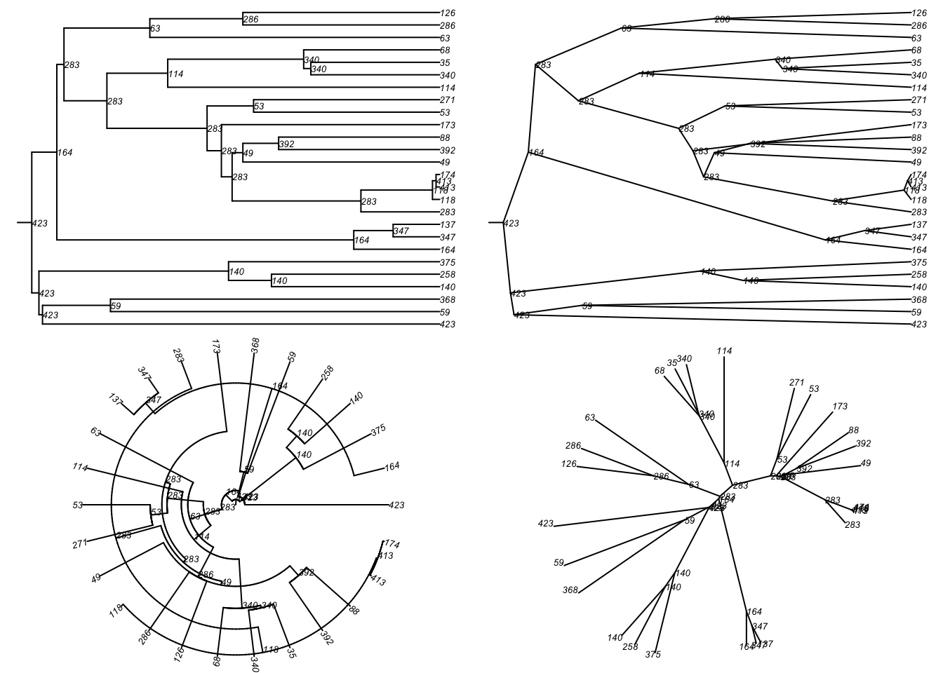
Last updated: 2022-07-07 with EpiModel v2.3.0