Tutorial: SIS Epidemic Across a Dynamic Network
Day 3 | Network Modeling for Epidemics
EpiModel uses separable-temporal exponential-family random graph models (STERGMs) to estimate and simulate complete networks based on individual-level, dyad-level, and network-level patterns of density, degree, assortivity, and other features influencing edge formation and dissolution. Building and simulating network-based epidemic models in EpiModel is a multi-step process, starting with estimation of a temporal ERGM and continuing with simulation of a dynamic network and epidemic processes on top of that network.
In this tutorial, we work through a model of a Susceptible-Infected-Susceptible (SIS) epidemic. One example of an SIS disease would be a bacterial sexually transmitted infection such as Gonorrhea, in which persons may acquire infection from sexual contact with an infected partner, and then recover from infection either through natural clearance or through antibiotic treatment.
We will use a simplifying assumption of a closed population, in which there are no entries or exits from the network; this may be justified by the short time span over which the epidemic will be simulated.
To get started, load the EpiModel library.
library(EpiModel)Network Model Estimation
The first step in our network model is to specify a network
structure, including features like size and nodal attributes. The
network_initialize function creates an object of class
network. Below we show an example of initializing a network
of 500 nodes, with no edges between them at the start. Edges represent
sexual partnerships (mutual person-to-person contact), so this is an
undirected network.
nw <- network_initialize(n = 500)The sizes of the networks represented in this workshop are smaller than what might be used for a research-level model, mostly for computational efficiency. Larger network sizes over longer time intervals are typically used for research purposes.
Model Parameterization
This example will start simple, with a formula that represents the
network density and the level of concurrency (overlapping sexual
partnerships) in the population. This is a dyad-dependent ERGM,
since the probability of edge formation between any two nodes depends on
the existence of edges between those nodes and other nodes. The
concurrent term is defined as the number of nodes with at least two
partners at any time. Following the notation of the tergm
package, we specify this using a right-hand side (RHS) formula. In
addition to concurrency, we will use a constraint on the degree
distribution. This will cap the degree of any person at 3, with no nodes
allowed to have 4 or more ongoing partnerships. This type of constraint
could reflect a truncated sampling scheme for partnerships within a
survey (e.g., persons only asked about their 3 most recent partners), or
a model assumption about limits of human activity.
formation <- ~edges + concurrent + degrange(from = 4)Target statistics will be the input mechanism for formation model
terms. The edges term will be a function of mean degree, or
the average number of ongoing partnerships. With an arbitrarily
specified mean degree of 0.7, the corresponding target statistic is 175:
\(edges = mean \ degree \times
\frac{N}{2}\).
We will also specify that 22% of persons exhibit concurrency (this is slightly higher than the 16% expected in a Poisson model conditional on that mean degree). The target statistic for the number of persons with a momentary degree of 4 or more is 0, reflecting our assumed constraint.
target.stats <- c(175, 110, 0)The dissolution model is parameterized from a mean
partnership duration estimated from cross-sectional egocentric data.
Dissolution models differ from formation models in two respects. First,
the dissolution models are not estimated in an ERGM but instead passed
in as a fixed coefficient conditional on which the formation model is to
be estimated. The dissolution model terms are calculated analytically
using the dissolution_coefs function, the output of which
is passed into the netest model estimation function.
Second, whereas formation models may be arbitrarily complex, dissolution
models are limited to a set of dyad-independent models; these are listed
in the dissolution_coefs function help page. The model we
will use is an edges-only model, implying a homogeneous probability of
dissolution for all partnerships in the network. The average duration of
these partnerships will be specified at 50 time steps, which will be
days in our model.
coef.diss <- dissolution_coefs(dissolution = ~offset(edges), duration = 50)
coef.diss
Dissolution Coefficients
=======================
Dissolution Model: ~offset(edges)
Target Statistics: 50
Crude Coefficient: 3.89182
Mortality/Exit Rate: 0
Adjusted Coefficient: 3.89182The output from this function indicates both an adjusted and crude coefficient. In this case, they are equivalent. Upcoming workshop material will showcase when they differ as result of exits from the network.
Model Estimation and Diagnostics
In EpiModel, network model estimation is performed with the
netest function, which is a wrapper around the estimation
functions in the ergm and tergm packages. The
function arguments are as follows:
function (nw, formation, target.stats, coef.diss, constraints,
    coef.form = NULL, edapprox = TRUE, set.control.ergm, set.control.stergm,
    set.control.tergm, verbose = FALSE, nested.edapprox = TRUE,
    ...)
NULL
The four arguments that must be specified with each function call are:
nw: an initialized empty network.formation: a RHS formation formula..target.stats: target statistics for the formation model.coef.diss: output object fromdissolution_coefs, containing the dissolution coefficients.
Other arguments that may be helpful to understand when getting started are:
constraints: this is another way of inputting model constraints (seehelp("ergm")).coef.form: sets the coefficient values of any offset terms in the formation model (those that are not explicitly estimated but fixed).edapprox: selects the dynamic estimation method. IfTRUE, uses the direct method, otherwise the approximation method.- Direct method: uses the functionality of the
tergmpackage to estimate the separable formation and dissolution models for the network. This is often not used because of computational time. - Approximation method: uses
ergmestimation for a cross-sectional network (the prevalence of edges) with an analytic adjustment of the edges coefficient to account for dissolution (i.e., transformation from prevalence to incidence). This approximation method may introduce bias into estimation in certain cases (high density and short durations) but these are typically not a concern for the low density cases in epidemiologically relevant networks.
- Direct method: uses the functionality of the
Estimation
Because we have a dyad-dependent model, MCMC will be used to estimate the coefficients of the model given the target statistics.
est <- netest(nw, formation, target.stats, coef.diss)Diagnostics
There are two forms of model diagnostics for a dynamic ERGM fit with
netest: static and dynamic diagnostics. When the
approximation method has been used, static diagnostics check the fit of
the cross-sectional model to target statistics. Dynamic diagnostics
check the fit of the model adjusted to account for edge dissolution.
When running a dynamic network simulation, it is good to start with the dynamic diagnostics, and if there are fit problems, work back to the static diagnostics to determine if the problem is due to the cross-sectional fit itself or with the dynamic adjustment (i.e., the approximation method). A proper fitting ERGM using the approximation method does not guarantee well-performing dynamic simulations.
Here we will examine dynamic diagnostics only. These are run with the
netdx function, which simulates from the model fit object
returned by netest. One must specify the number of
simulations from the dynamic model and the number of time steps per
simulation. Choice of both simulation parameters depends on the
stochasticity in the model, which is a function of network size, model
complexity, and other factors. The nwstats.formula contains
the network statistics to monitor in the diagnostics: it may contain
statistics in the formation model and also others. By default, it is the
formation model. Finally, we are keeping the “timed edgelist” with
keep.tedgelist.
dx <- netdx(est, nsims = 10, nsteps = 1000,
            nwstats.formula = ~edges + meandeg + degree(0:4) + concurrent,
            keep.tedgelist = TRUE)
We have also built in parallelization into the EpiModel simulation functions, so it is also possible to run multiple simulations at the same time using your computer’s multi-core design. You can find the number of cores in your system with:
parallel::detectCores()Then you can run the multi-core simulations by specifying
ncores (EpiModel will prevent you from specifying more
cores than you have available).
dx <- netdx(est, nsims = 10, nsteps = 1000, ncores = 4,
            nwstats.formula = ~edges + meandeg + degree(0:4) + concurrent,
            keep.tedgelist = TRUE)
Printing the object will show the object structure and diagnostics.
Both formation and duration diagnostics show a good fit relative to
their targets. For the formation diagnostics, the mean statistics are
the mean of the cross sectional statistics at each time step across all
simulations. The Pct Diff column shows the relative
difference between the mean and targets. There are two forms of
dissolution diagnostics. The edge duration row shows the mean duration
of partnerships across the simulations; it tends to be lower than the
target unless the diagnostic simulation interval is very long since its
average includes a burn-in period where all edges start at a duration of
zero (illustrated below in the plot). The next row shows the percent of
current edges dissolving at each time step, and is not subject to bias
related to burn-in. The percentage of edges dissolution is the inverse
of the expected duration: if the duration is 50 days, then we expect
that 1/50 (or 2%) to dissolve each day.
print(dx)EpiModel Network Diagnostics
=======================
Diagnostic Method: Dynamic
Simulations: 10
Time Steps per Sim: 1000
Formation Diagnostics
-----------------------
Target Sim Mean Pct Diff Sim SD
edges 175 176.586 0.906 13.530
meandeg NA 0.706 NA 0.054
degree0 NA 270.455 NA 15.182
degree1 NA 119.591 NA 10.146
degree2 NA 96.281 NA 10.718
degree3 NA 13.673 NA 3.750
degree4 NA 0.000 NA 0.000
concurrent 110 109.954 -0.042 11.841
deg4+ 0 NA NA NA
Duration Diagnostics
-----------------------
Target Sim Mean Pct Diff Sim SD
edges 50 49.85 -0.299 1.275
Dissolution Diagnostics
-----------------------
Target Sim Mean Pct Diff Sim SD
edges 0.02 0.02 0.244 0Plotting the diagnostics object will show the time series of the target statistics against any targets. The other options used here specify to smooth the mean lines, give them a thicker line width, and plot each statistic in a separate panel. The black dashed lines show the value of the target statistics for any terms in the model. Similar to the numeric summaries, the plots show a good fit over the time series.
plot(dx)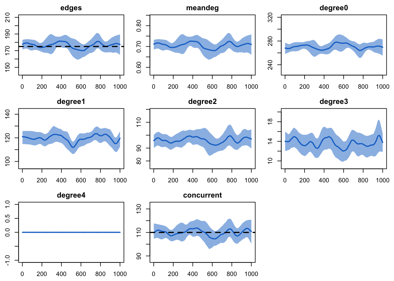
The simulated network statistics from diagnostic object may be
extracted into a data.frame with
get_nwstats.
nwstats1 <- get_nwstats(dx, sim = 1)
head(nwstats1, 20)
time sim edges meandeg degree0 degree1 degree2 degree3 degree4 concurrent
1 1 1 170 0.680 281 114 89 16 0 105
2 2 1 172 0.688 278 117 88 17 0 105
3 3 1 170 0.680 278 120 86 16 0 102
4 4 1 171 0.684 278 119 86 17 0 103
5 5 1 169 0.676 282 114 88 16 0 104
6 6 1 170 0.680 280 116 88 16 0 104
7 7 1 172 0.688 276 120 88 16 0 104
8 8 1 174 0.696 275 122 83 20 0 103
9 9 1 174 0.696 278 117 84 21 0 105
10 10 1 175 0.700 276 119 84 21 0 105
11 11 1 178 0.712 276 113 90 21 0 111
12 12 1 176 0.704 276 115 90 19 0 109
13 13 1 176 0.704 273 121 87 19 0 106
14 14 1 173 0.692 274 122 88 16 0 104
15 15 1 172 0.688 274 124 86 16 0 102
16 16 1 172 0.688 274 124 86 16 0 102
17 17 1 172 0.688 274 123 88 15 0 103
18 18 1 169 0.676 276 123 88 13 0 101
19 19 1 173 0.692 275 117 95 13 0 108
20 20 1 176 0.704 273 116 97 14 0 111The dissolution model fit may also be assessed with plots by
specifying either the duration or dissolution
type, as defined above. The duration diagnostic is based on the average
age of edges at each time step, up to that time step. An imputation
algorithm is used for left-censored edges (i.e., those that exist at
t1); you can turn off this imputation to see the effects of censoring
with duration.imputed = FALSE. Both metrics show a good fit
of the dissolution model to the target duration of 50 time steps.
par(mfrow = c(1, 2))
plot(dx, type = "duration")
plot(dx, type = "dissolution")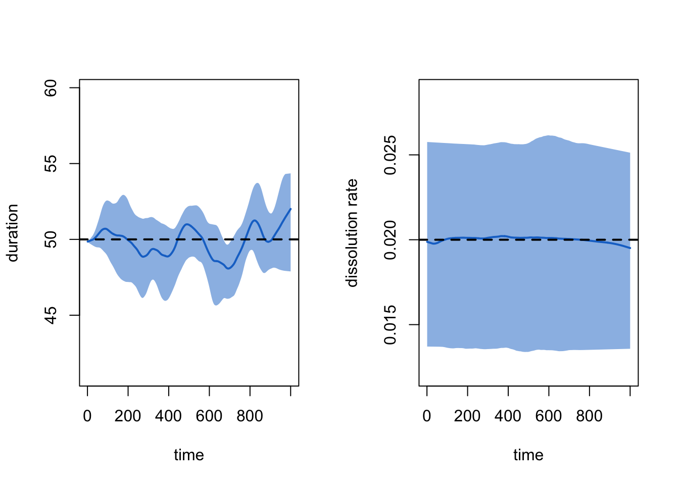
By inspecting the timed edgelist, we can see the burn-in period
directly with censoring of onset times. The as.data.frame
function is used to extract this edgelist object.
tel <- as.data.frame(dx, sim = 1)
head(tel, 20)
onset terminus tail head onset.censored terminus.censored duration edge.id
1 0 197 1 101 TRUE FALSE 197 1
2 0 145 2 142 TRUE FALSE 145 2
3 0 3 5 356 TRUE FALSE 3 3
4 0 19 5 454 TRUE FALSE 19 4
5 0 22 6 132 TRUE FALSE 22 5
6 0 148 6 387 TRUE FALSE 148 6
7 0 28 8 26 TRUE FALSE 28 7
8 0 30 8 316 TRUE FALSE 30 8
9 541 568 8 316 FALSE FALSE 27 8
10 0 45 9 100 TRUE FALSE 45 9
11 0 16 9 386 TRUE FALSE 16 10
12 0 34 14 121 TRUE FALSE 34 11
13 0 131 14 474 TRUE FALSE 131 12
14 0 29 20 409 TRUE FALSE 29 13
15 0 62 26 464 TRUE FALSE 62 14
16 0 80 28 60 TRUE FALSE 80 15
17 0 65 28 366 TRUE FALSE 65 16
18 0 29 30 146 TRUE FALSE 29 17
19 0 13 30 214 TRUE FALSE 13 18
20 0 81 32 115 TRUE FALSE 81 19If the model diagnostics had suggested a poor fit, then additional
diagnostics and fitting would be necessary. If using the approximation
method, one should first start by running the cross-sectional
diagnostics (setting dynamic to FALSE in
netdx). Note that the number of simulations may be very
large here and there are no time steps specified
because each simulation is a cross-sectional network.
dx.static <- netdx(est, nsims = 10000, dynamic = FALSE)
print(dx.static)
The plots now represent individual simulations from an MCMC chain, rather than time steps.
par(mfrow = c(1,1))
plot(dx.static, sim.lines = TRUE, sim.lwd = 0.1)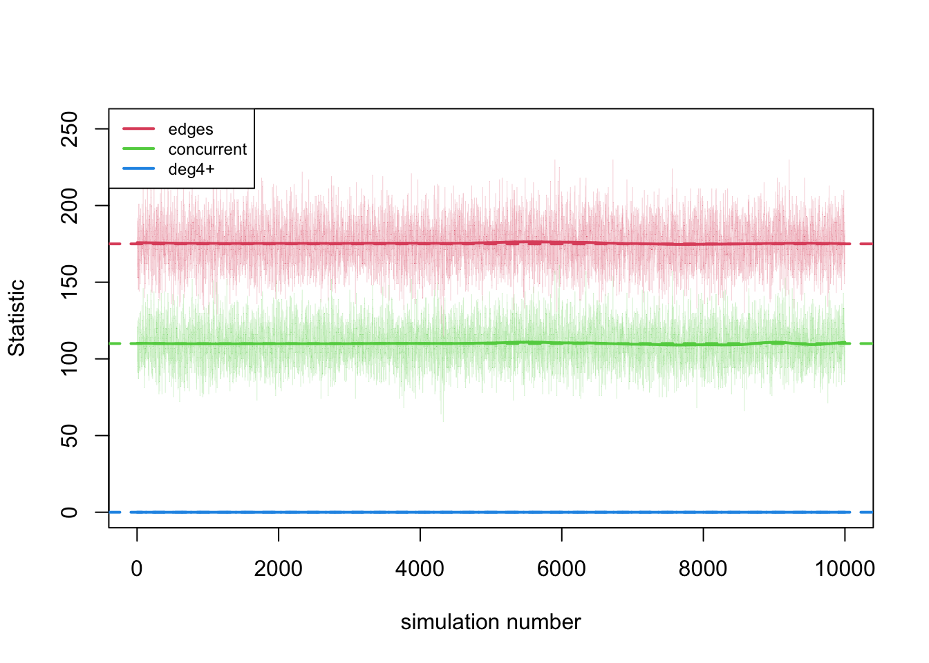
This lack of temporality is now evident when looking at the raw data.
nwstats2 <- get_nwstats(dx.static)
head(nwstats2, 20)
sim edges concurrent deg4+
1 1 192 125 0
2 2 177 113 0
3 3 172 98 0
4 4 179 121 0
5 5 153 91 0
6 6 158 94 0
7 7 162 94 0
8 8 153 92 0
9 9 165 95 0
10 10 171 97 0
11 11 160 99 0
12 12 177 106 0
13 13 190 121 0
14 14 188 118 0
15 15 161 95 0
16 16 162 102 0
17 17 167 104 0
18 18 145 87 0
19 19 186 111 0
20 20 170 111 0If the cross-sectional model fits well but the dynamic model does
not, then a full STERGM estimation may be necessary (using
edapprox = TRUE). If the cross-sectional model does not fit
well, different control parameters for the ERGM estimation may be
necessary (see the help file for netdx for
instructions).
Epidemic Simulation
EpiModel simulates disease epidemics over dynamic networks by integrating dynamic model simulations with the simulation of other epidemiological processes such as disease transmission and recovery. Like the network model simulations, these processes are also simulated stochastically so that the range of potential outcomes under the model specifications is estimated.
The specification of epidemiological processes to model may be arbitrarily complex, but EpiModel includes a number of “built-in” model types within the software. Additional components will be programmed and plugged into the simulation API (just like any epidemic model); we will start to cover that tomorrow. Here, we will start simple with an SIS epidemic using this built-in functionality. This is starting point to what you can do in EpiModel!
Epidemic Model Parameters
Our SIS model will rely on three parameters. The act rate is the number of sexual acts that occur within a partnership each time unit. The overall frequency of acts per person per unit time is a function of the incidence rate of partnerships and this act rate parameter. The infection probability is the risk of transmission given contact with an infected person. The recovery rate for an SIS epidemic is the speed at which infected persons become susceptible again. For a bacterial STI like gonorrhea, this may be a function of biological attributes like sex or use of therapeutic agents like antibiotics.
EpiModel uses three helper functions to input epidemic parameters,
initial conditions, and other control settings for the epidemic model.
First, we use the param.net function to input the per-act
transmission probability in inf.prob and the number of acts
per partnership per unit time in act.rate. The recovery
rate implies that the average duration of disease is 10 days
(1/rec.rate).
param <- param.net(inf.prob = 0.4, act.rate = 2, rec.rate = 0.1)For initial conditions in this model, we only need to specify the number of infected persons at the outset of the epidemic. The remaining persons in the network will be classified as disease susceptible.
init <- init.net(i.num = 10)The control settings specify the structural elements of the model.
These include the disease type, number of simulations, and number of
time steps per simulation. (Here again we could use the model multi-core
functionality by specifying an ncores value, but these
models run so quickly that it’s not necessary.)
control <- control.net(type = "SIS", nsims = 5, nsteps = 500)Simulating the Epidemic Model
Once the model has been parameterized, simulating the model is
straightforward. One must pass the fitted network model object from
netest along with the parameters, initial conditions, and
control settings to the netsim function. With a no-feedback
model like this (i.e., there are no vital dynamics parameters), the full
dynamic network time series is simulated at the start of each epidemic
simulation, and then the epidemiological processes are simulated over
that structure.
sim <- netsim(est, param, init, control)Printing the model output lists the inputs and outputs of the model.
The output includes the sizes of the compartments (s.num is
the number susceptible and i.num is the number infected)
and flows (si.flow is the number of infections and
is.flow is the number of recoveries). Methods for
extracting this output is discussed below.
print(sim)EpiModel Simulation
=======================
Model class: netsim
Simulation Summary
-----------------------
Model type: SIS
No. simulations: 5
No. time steps: 500
No. NW groups: 1
Fixed Parameters
---------------------------
inf.prob = 0.4
act.rate = 2
rec.rate = 0.1
groups = 1
Model Output
-----------------------
Variables: s.num i.num num si.flow is.flow
Networks: sim1 ... sim5
Transmissions: sim1 ... sim5
Formation Diagnostics
-----------------------
Target Sim Mean Pct Diff Sim SD
edges 175 173.513 -0.850 13.935
concurrent 110 108.208 -1.629 12.566
deg4+ 0 0.000 NaN 0.000
Dissolution Diagnostics
-----------------------
Target Sim Mean Pct Diff Sim SD
edges 0.02 NaN NaN NAModel Analysis
Now the the model has been simulated, the next step is to analyze the data. This includes plotting the epidemiological output, the networks over time, and extracting other raw data.
Epidemic Plots
Plotting the output from the epidemic model using the default arguments will display the size of the compartments in the model across simulations. The means across simulations at each time step are plotted with lines, and the polygon band shows the inter-quartile range across simulations.
par(mfrow = c(1, 1))
plot(sim)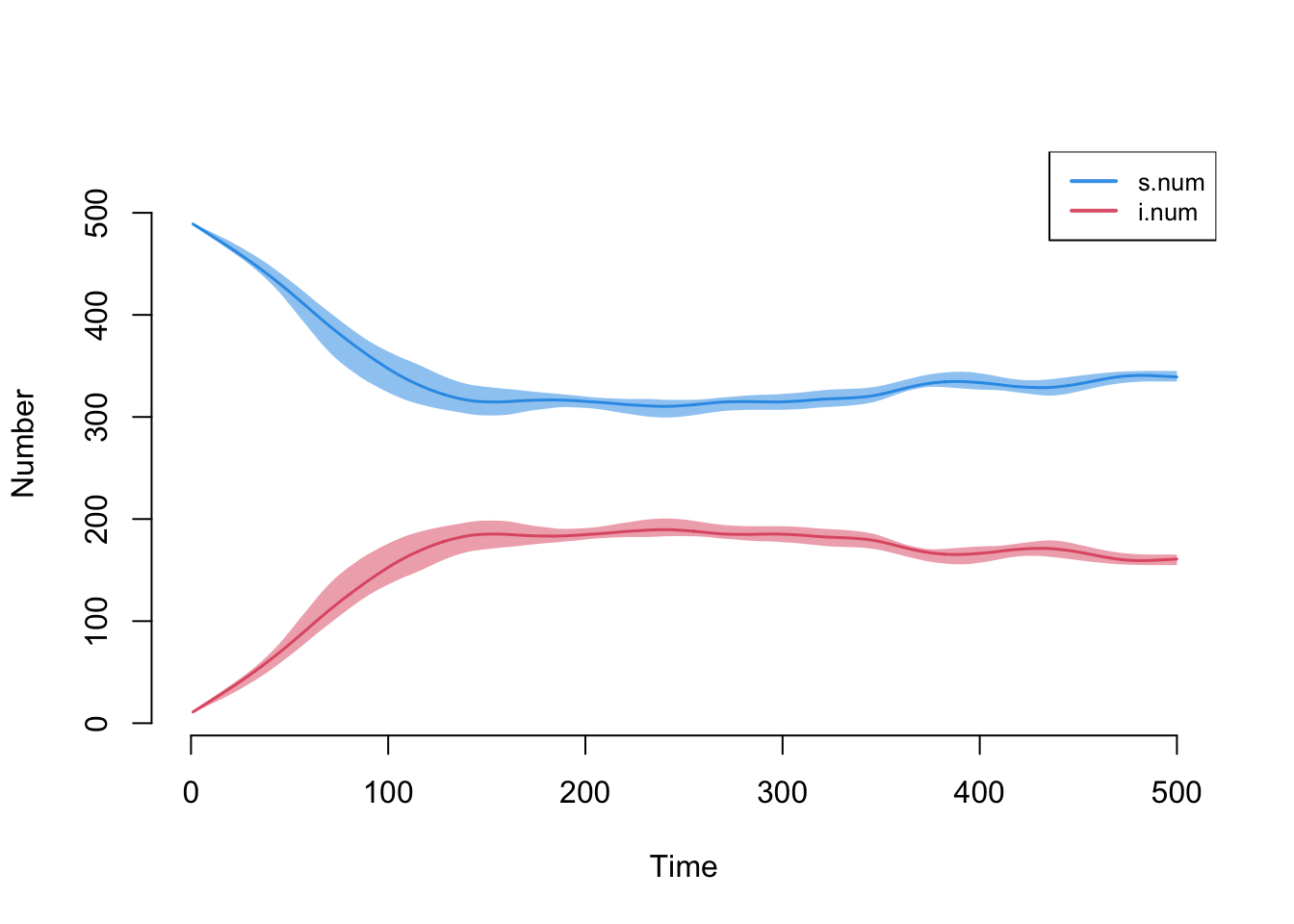
Graphical elements may be toggled on and off. The
popfrac argument specifies whether to use the absolute size
of compartments versus proportions.
par(mfrow = c(1, 2))
plot(sim, sim.lines = TRUE, mean.line = FALSE, qnts = FALSE, popfrac = TRUE)
plot(sim, mean.smooth = FALSE, qnts = 1, qnts.smooth = FALSE, popfrac = TRUE)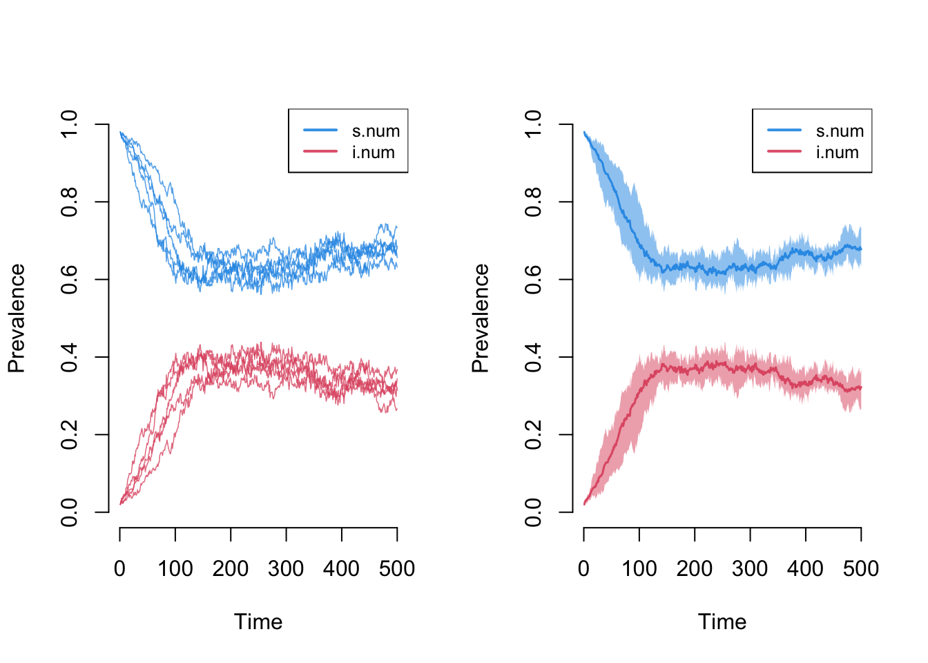
Whereas the default will print the compartment proportions, other
elements of the simulation may be plotted by name with the
y argument. Here we plot both flow sizes using smoothed
means, which converge at model equilibrium by the end of the time
series.
par(mfrow = c(1,1))
plot(sim, y = c("si.flow", "is.flow"), qnts = FALSE,
     ylim = c(0, 25), legend = TRUE, main = "Flow Sizes")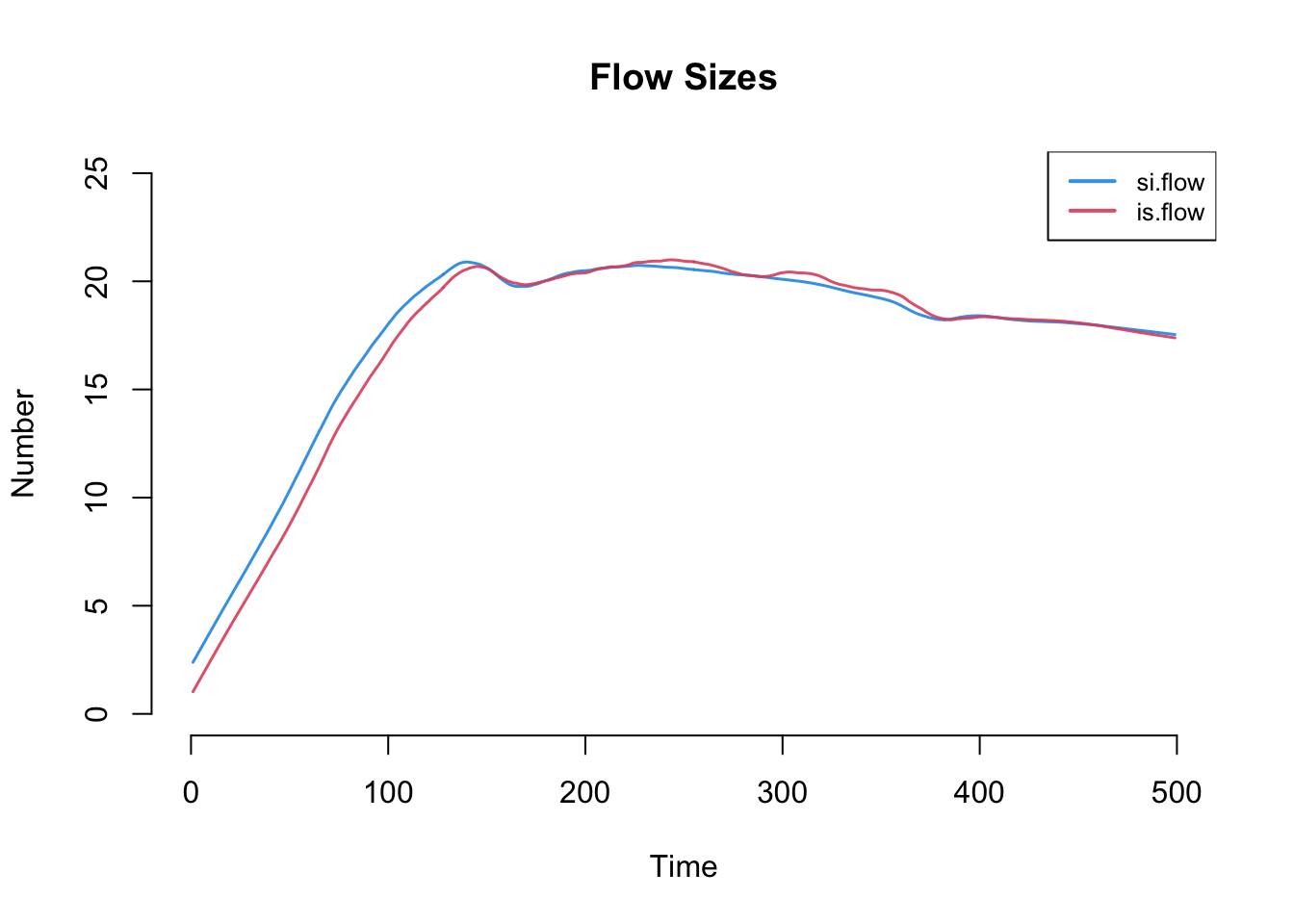
Network Plots
Another available plot type is a network plot to visualize the
individual nodes and edges at a specific time point. Network plots are
output by setting the type parameter to
"network". To plot the disease infection status on the
nodes, use the col.status argument: blue indicates
susceptible and red infected. It is necessary to specify both a time
step and a simulation number to plot these networks.
par(mfrow = c(1, 2), mar = c(0, 0, 0, 0))
plot(sim, type = "network", col.status = TRUE, at = 1, sims = 1)
plot(sim, type = "network", col.status = TRUE, at = 500, sims = 1)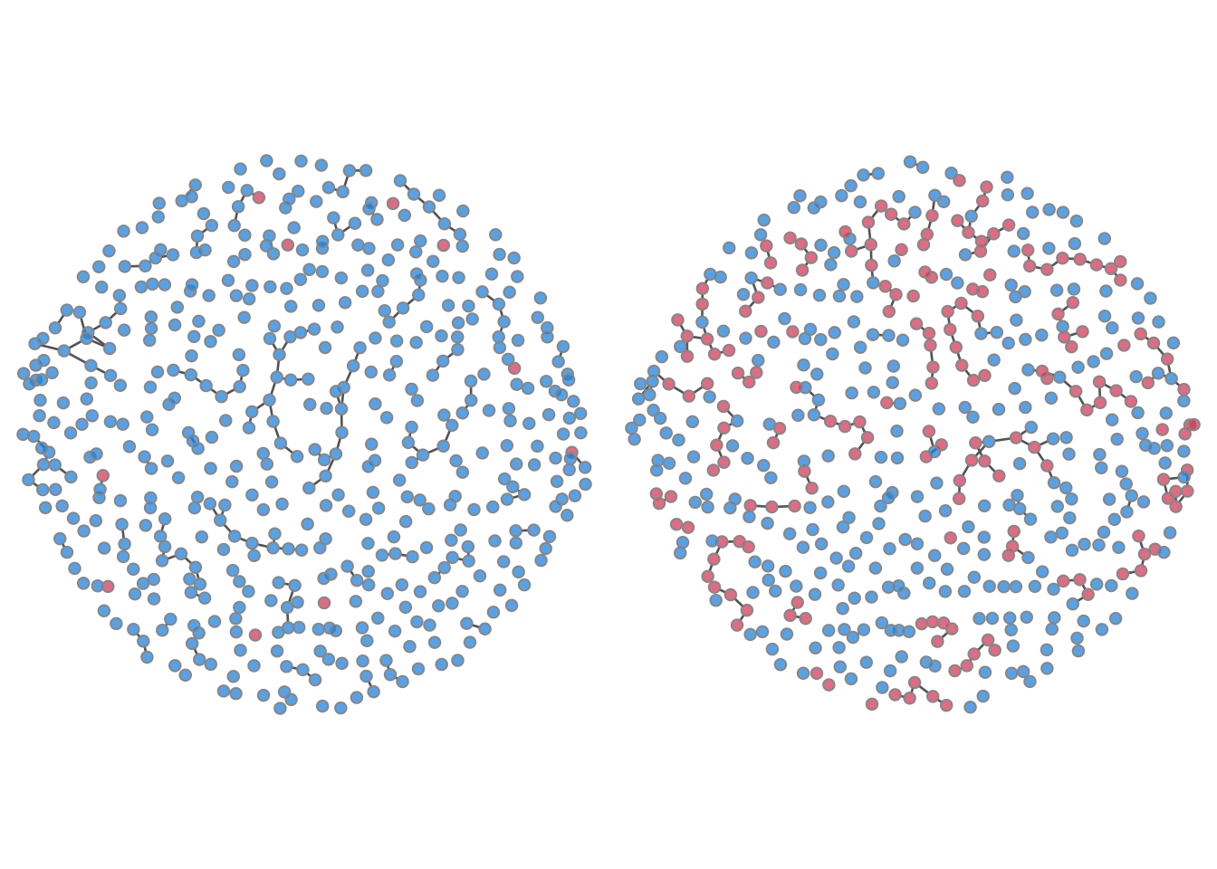
Time-Specific Model Summaries
The summary function with the output of netsim will show
the model statistics at a specific time step. Here we output the
statistics at the final time step, where roughly two-thirds of the
population are infected.
summary(sim, at = 500)
EpiModel Summary
=======================
Model class: netsim

Simulation Details
-----------------------
Model type: SIS
No. simulations: 5
No. time steps: 500
No. NW groups: 1

Model Statistics
------------------------------
Time: 500
------------------------------
           mean      sd    pct
Suscept.  338.8  19.045  0.678
Infect.   161.2  19.045  0.322
Total     500.0   0.000  1.000
S -> I     16.2   4.207     NA
I -> S     15.2   3.493     NA
------------------------------
Data Extraction
The as.data.frame function may be used to extract the
model output into a data frame object for easy analysis outside of the
built-in EpiModel functions. The function default will output the raw
data for all simulations for each time step.
df <- as.data.frame(sim)
head(df, 10)
sim time s.num i.num num si.flow is.flow
1 1 1 490 10 500 NA NA
2 1 2 487 13 500 4 1
3 1 3 487 13 500 2 2
4 1 4 488 12 500 1 2
5 1 5 489 11 500 0 1
6 1 6 487 13 500 2 0
7 1 7 487 13 500 3 3
8 1 8 485 15 500 3 1
9 1 9 483 17 500 3 1
10 1 10 483 17 500 3 3tail(df, 10) sim time s.num i.num num si.flow is.flow
2491 5 491 355 145 500 16 16
2492 5 492 352 148 500 19 16
2493 5 493 357 143 500 18 23
2494 5 494 353 147 500 17 13
2495 5 495 358 142 500 12 17
2496 5 496 364 136 500 16 22
2497 5 497 365 135 500 19 20
2498 5 498 369 131 500 17 21
2499 5 499 367 133 500 19 17
2500 5 500 367 133 500 15 15The out argument may be changed to specify the output of
means across the models (with out = "mean"). The output
below shows all compartment and flow sizes as integers, reinforcing this
as an individual-level model.
df <- as.data.frame(sim, out = "mean")
head(df, 10)
time s.num i.num num si.flow is.flow
1 1 490.0 10.0 500 NaN NaN
2 2 486.8 13.2 500 4.6 1.4
3 3 485.0 15.0 500 2.8 1.0
4 4 484.6 15.4 500 3.0 2.6
5 5 484.0 16.0 500 1.6 1.0
6 6 483.6 16.4 500 1.8 1.4
7 7 481.8 18.2 500 3.2 1.4
8 8 481.2 18.8 500 2.2 1.6
9 9 480.0 20.0 500 3.2 2.0
10 10 479.8 20.2 500 3.2 3.0tail(df, 10) time s.num i.num num si.flow is.flow
491 491 339.2 160.8 500 18.2 17.6
492 492 338.6 161.4 500 17.4 16.8
493 493 339.8 160.2 500 19.6 20.8
494 494 339.4 160.6 500 19.0 18.6
495 495 338.2 161.8 500 16.4 15.2
496 496 337.6 162.4 500 18.0 17.4
497 497 340.2 159.8 500 18.2 20.8
498 498 341.6 158.4 500 19.2 20.6
499 499 339.8 160.2 500 20.8 19.0
500 500 338.8 161.2 500 16.2 15.2The networkDynamic objects are stored in the
netsim object, and may be extracted with the
get_network function. By default the dynamic networks are
saved, and contain the full edge history for every node that has existed
in the network, along with the disease status history of those
nodes.
nw1 <- get_network(sim, sim = 1)
nw1
NetworkDynamic properties:
distinct change times: 502
maximal time range: -Inf until Inf
Dynamic (TEA) attributes:
Vertex TEAs: testatus.active
Includes optional net.obs.period attribute:
Network observation period info:
Number of observation spells: 2
Maximal time range observed: 1 until 501
Temporal mode: discrete
Time unit: step
Suggested time increment: 1
Network attributes:
vertices = 500
directed = FALSE
hyper = FALSE
loops = FALSE
multiple = FALSE
bipartite = FALSE
net.obs.period: (not shown)
total edges= 1889
missing edges= 0
non-missing edges= 1889
Vertex attribute names:
active status testatus.active vertex.names
Edge attribute names not shown One thing you can do with that network dynamic object is to extract the timed edgelist of all ties that existed for that simulation.
nwdf <- as.data.frame(nw1)
head(nwdf, 25)
onset terminus tail head onset.censored terminus.censored duration edge.id
1 1 44 1 293 TRUE FALSE 43 1
2 1 72 3 87 TRUE FALSE 71 2
3 1 16 5 71 TRUE FALSE 15 3
4 1 53 5 133 TRUE FALSE 52 4
5 1 47 7 184 TRUE FALSE 46 5
6 1 2 10 126 TRUE FALSE 1 6
7 1 24 10 214 TRUE FALSE 23 7
8 129 138 10 214 FALSE FALSE 9 7
9 1 38 13 420 TRUE FALSE 37 8
10 1 175 16 244 TRUE FALSE 174 9
11 1 6 16 420 TRUE FALSE 5 10
12 1 30 22 391 TRUE FALSE 29 12
13 1 46 22 406 TRUE FALSE 45 13
14 1 71 25 60 TRUE FALSE 70 14
15 1 64 28 81 TRUE FALSE 63 15
16 1 87 31 346 TRUE FALSE 86 17
17 1 32 32 69 TRUE FALSE 31 18
18 1 9 36 189 TRUE FALSE 8 19
19 1 55 38 58 TRUE FALSE 54 20
20 1 32 39 64 TRUE FALSE 31 21
21 1 100 44 241 TRUE FALSE 99 22
22 1 43 44 336 TRUE FALSE 42 23
23 1 21 46 361 TRUE FALSE 20 24
24 1 20 47 298 TRUE FALSE 19 25
25 288 290 47 298 FALSE FALSE 2 25A matrix is stored that records some key details about each
transmission event that occurred. Shown below are the first 10
transmission events for simulation number 1. The sus column
shows the unique ID of the previously susceptible, newly infected node
in the event. The inf column shows the ID of the
transmitting node. The other columns show the duration of the
transmitting node’s infection at the time of transmission, the per-act
transmission probability, act rate during the transmission, and final
per-partnership transmission rate (which is the per-act probability
raised to the number of acts).
tm1 <- get_transmat(sim, sim = 1)
head(tm1, 10)
at sus inf infDur transProb actRate finalProb
1 2 198 251 28 0.4 2 0.64
2 2 325 321 2 0.4 2 0.64
3 2 490 352 3 0.4 2 0.64
4 2 462 447 10 0.4 2 0.64
5 3 90 447 11 0.4 2 0.64
6 3 325 321 3 0.4 2 0.64
7 4 447 90 1 0.4 2 0.64
8 6 106 490 4 0.4 2 0.64
9 6 447 90 3 0.4 2 0.64
10 7 123 342 5 0.4 2 0.64Data Exporting and Plotting with ggplot
We built in plotting methods directly for netsim class
objects so you can easily plot multiple types of summary statistics from
the simulated model object. However, if you prefer an external plotting
tool in R, such as ggplot, it is easy to extract the data
in tidy format for analysis and plotting. Here is an
example how to do so for out model above. See the help for the ggplot if
you are unfamiliar with this syntax.
df <- as.data.frame(sim)
df.mean <- as.data.frame(sim, out = "mean")

library(ggplot2)
Attaching package: 'ggplot2'The following object is masked from 'package:latticeExtra':
layerggplot() +
geom_line(data = df, mapping = aes(time, i.num, group = sim), alpha = 0.25,
lwd = 0.25, color = "firebrick") +
geom_bands(data = df, mapping = aes(time, i.num),
lower = 0.1, upper = 0.9, fill = "firebrick") +
geom_line(data = df.mean, mapping = aes(time, i.num)) +
theme_minimal()
Last updated: 2022-07-07 with EpiModel v2.3.0