Tutorial: Adding a Latent Stage to Make an SEIR Model

EpiModel includes an integrated SIR model, but here we show how to model an SEIR disease like COVID-19. The E compartment in this disease is an exposed state in which a person has been infected but is not infectious to others. Some infectious diseases have this latent non-infectious stage, and in general it provides a general framework for transmission risk that is dependent on one’s stage of disease progression.

Setup

First start by loading EpiModel and clearing your global environment.

library(EpiModel)
rm(list = ls())

EpiModel Model Extensions

Conceptualization

The first step to any EpiModel extension model is to conceptually identify what new functionality, above and beyond the built-in models, is desired and where that functionality should be added. There are often many “right” answers to these questions, and this aspect is only learned over time. But in general, it is helpful to map out a model extension on a state/flow diagram to pinpoint where the additions should be concentrated.

SIR Module Set

In this particular model, we will be adding a new disease state that occurs in between the susceptible disease state and an infectious disease state in an SIR model. The standard, built-in SIR model in EpiModel uses set modules (elements of the model), each with its own set of associated functions (the realization of those elements in code). For any built-in model, you can see what set of modules and functions have been used by running the simulation with netsim and then printing the output.

nw <- network_initialize(n = 100)
formation <- ~edges
target.stats <- 50
coef.diss <- dissolution_coefs(dissolution = ~offset(edges), duration = 20)
est1 <- netest(nw, formation, target.stats, coef.diss, verbose = FALSE)
param <- param.net(inf.prob = 0.3, rec.rate = 0.1)
init <- init.net(i.num = 10, r.num = 0)
control <- control.net(type = "SIR", nsteps = 25, nsims = 1, verbose = FALSE)
mod1 <- netsim(est1, param, init, control)
mod1

EpiModel Simulation
=======================
Model class: netsim

Simulation Summary
-----------------------
Model type: SIR
No. simulations: 1
No. time steps: 25
No. NW groups: 1

Fixed Parameters
---------------------------
inf.prob = 0.3
rec.rate = 0.1
act.rate = 1
groups = 1

Model Output
-----------------------
Variables: s.num i.num r.num num si.flow ir.flow
Networks: sim1
Transmissions: sim1

Formation Diagnostics
----------------------- 
      Target Sim Mean Pct Diff Sim SD
edges     50    41.32   -17.36  3.637


Dissolution Diagnostics
----------------------- 
      Target Sim Mean Pct Diff Sim SD
edges   0.05      NaN      NaN     NA

Module Classes

This includes a series of modules, which we classify into Standard and Flexible modules as shown on the table below. Any modules may be modified, but standard modules are those that are typically not modified because they generalize the core internal processes for simulation object generation, network resimulation, and epidemic bookkeeping. Flexible modules, in contrast, are those that are likely necessary to modify for an EpiModel extension.

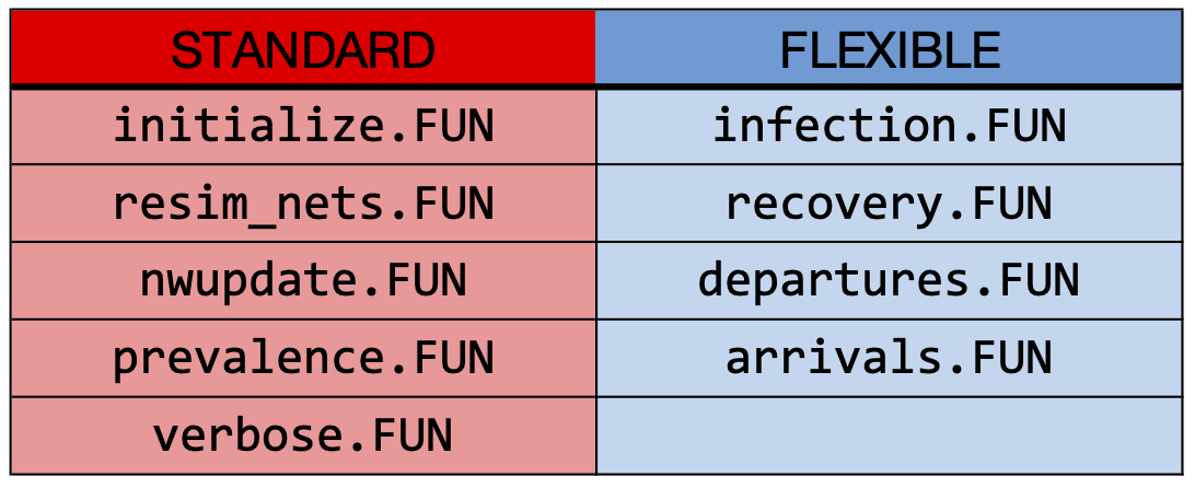
In the example above, we used all of these modules except the arrivals and departures modules because we had a closed population. In addition to these set of built-in modules, any user can add more modules to this set, depending on what is needed. Again, this involves some conceptualization of how to organize the model processes, including whether those processes are similar to the built-in modules or something new.

Modules vs. Functions

All modules have associated functions, and these are passed into the epidemic model run in netsim through control.net. Printing out the arguments for this function, you will see that each of the standard modules have default associated functions as inputs, and flexible modules have a default of NULL.

args(control.net)

function (type, nsteps, start = 1, nsims = 1, ncores = 1, resimulate.network = FALSE, 
    tergmLite = FALSE, cumulative.edgelist = FALSE, truncate.el.cuml = 0, 
    attr.rules, epi.by, initialize.FUN = initialize.net, resim_nets.FUN = resim_nets, 
    infection.FUN = NULL, recovery.FUN = NULL, departures.FUN = NULL, 
    arrivals.FUN = NULL, nwupdate.FUN = nwupdate.net, prevalence.FUN = prevalence.net, 
    verbose.FUN = verbose.net, module.order = NULL, save.nwstats = TRUE, 
    nwstats.formula = "formation", save.transmat = TRUE, save.network, 
    save.other, verbose = TRUE, verbose.int = 1, skip.check = FALSE, 
    raw.output = FALSE, tergmLite.track.duration = FALSE, set.control.ergm = control.simulate.formula(MCMC.burnin = 2e+05), 
    set.control.stergm = NULL, set.control.tergm = control.simulate.formula.tergm(), 
    ...) 
NULL

For built-in models, EpiModel selects which modules are needed based on the model parameters and initial conditions. For each time step, the modules run in the order in which they are specified in the output here; this also matches the order in which they are listed in control.net.

Built-in Functions as Templates

Any of the built-in functions associated with flexible modules are intended to be templates for user inspection and extension for research-level models. So, for example, mod1 above shows that infection.net was used as the infection module. That function has a help page briefly describing what it does. And you can also inspect the function contents with:

View(infection.net)

We’ll use an edited down version of that function, with some additional explanation, below. In addition, the disease progression state transition within an SIR model (and an SIS model too) is handled by the recovery module, with an associated recovery.net function.

View(recovery.net)

We will use an edited down version of that function as a template for a new, more general disease progression module.

The EpiModel API

All EpiModel module functions have a set of shared design requirements. This set of requirements defines the EpiModel Application Programming Interface (API) for extension. The best way to learn this is through a concrete example like this, but here are the general API rules:

1. Each module has an associated R function, the general design of which is:

fx <- function(dat, at) {
  
  ## function processes that update dat
  
  return(dat)
}

The function takes an object called dat, which is the master data object passed around by netsim, performs some processes (e.g., infection, recovery, aging, interventions), updates the dat object, and then returns that object. The other input argument to each function must be at, which is a time step counter.

2. Data are stored on the dat object in a particular way: in sublists that are organized by category. The main categories of data to interact with include model inputs (parameters, initial conditions, and controls) from those three associated input functions; nodal attributes (e.g., an individual disease status for each person); and summary statistics (e.g., the disease prevalence at at time step). There are accessor functions for reading (these are the get_ functions) and writing (these are the set_ functions) to the dat object in the appropriate place.

3. The typical function design involves three steps: a) reading the relevant inputs from the dat object; b) performing some micro-level process on the nodes that is usually a function of fixed parameters and time-varying nodal attributes; c) writing the updated objects back on to the dat object.

Let’s see how this API works by extending our infection and recovery functions to transition an SIR model into an SEIR model.

Infection Module

The built-in infection module for an SIR model performs the following functions listed in the function below. The core process is determining which edges are eligible for a disease transmission to occur, and then randomly simulating that transmission process. Why is it necessary to update the infection function for an SEIR model? Because an SIR involves a transition between S and I disease statuses when a new infection occurs, but an SEIR model involves a transition between S and E disease statuses. It’s a small, but important change. Here’s the full modified function, with embedded comments. Note that we can use the browser function to run this function in debug mode by uncommenting the third line (we will demonstrate this).

infect <- function(dat, at) {

  ## Uncomment this to run environment interactively
  # browser()

  ## Attributes ##
  active <- get_attr(dat, "active")
  status <- get_attr(dat, "status")
  infTime <- get_attr(dat, "infTime")

  ## Parameters ##
  inf.prob <- get_param(dat, "inf.prob")
  act.rate <- get_param(dat, "act.rate")

  ## Find infected nodes ##
  idsInf <- which(active == 1 & status == "i")
  nActive <- sum(active == 1)
  nElig <- length(idsInf)

  ## Initialize default incidence at 0 ##
  nInf <- 0

  ## If any infected nodes, proceed with transmission ##
  if (nElig > 0 && nElig < nActive) {

    ## Look up discordant edgelist ##
    del <- discord_edgelist(dat, at)

    ## If any discordant pairs, proceed ##
    if (!(is.null(del))) {

      # Set parameters on discordant edgelist data frame
      del$transProb <- inf.prob
      del$actRate <- act.rate
      del$finalProb <- 1 - (1 - del$transProb)^del$actRate

      # Stochastic transmission process
      transmit <- rbinom(nrow(del), 1, del$finalProb)

      # Keep rows where transmission occurred
      del <- del[which(transmit == 1), ]

      # Look up new ids if any transmissions occurred
      idsNewInf <- unique(del$sus)
      nInf <- length(idsNewInf)

      # Set new attributes and transmission matrix
      if (nInf > 0) {
        status[idsNewInf] <- "e"
        infTime[idsNewInf] <- at
        dat <- set_attr(dat, "status", status)
        dat <- set_attr(dat, "infTime", infTime)

        dat <- set_transmat(dat, del, at)
  
      }
    }
  }

  ## Save summary statistic for S->E flow
  dat <- set_epi(dat, "se.flow", at, nInf)

  return(dat)
}

Each step is relatively self-explanatory with the comments, but we will run this interactively at the end of this tutorial to step through the updated data structures. Infection is one of the more complex processes because it involves a dyadic process (a contact between an S and I node). That involves a construction of a discordant edgelist; that is, a list of edges in which there is a disease discordant dyad.

The main point here is: we have made a change to the infection module function, and it consists of updating the disease status of a newly infected persons to "e" instead of "i". Additionally, we are tracking a new summary statistic, se.flow that tracks the size of the flow from S to E based on the number of new infected, nInf at the time step.

Progression Module

Next up is the disease progression module. Here, we have generalized the built-in recovery module function to handle two disease progression transitions after infection: E to I (latent to infectious stages) and I to R (infectious to recovered stages). Like many individual-level transitions, this involves flipping a weighted coin with rbinom: this performs a series of random Bernoulli draws based on the specified parameters. Here is the full model function.

progress <- function(dat, at) {

  ## Uncomment this to function environment interactively
  # browser()

  ## Attributes ##
  active <- get_attr(dat, "active")
  status <- get_attr(dat, "status")

  ## Parameters ##
  ei.rate <- get_param(dat, "ei.rate")
  ir.rate <- get_param(dat, "ir.rate")

  ## E to I progression process ##
  nInf <- 0
  idsEligInf <- which(active == 1 & status == "e")
  nEligInf <- length(idsEligInf)

  if (nEligInf > 0) {
    vecInf <- which(rbinom(nEligInf, 1, ei.rate) == 1)
    if (length(vecInf) > 0) {
      idsInf <- idsEligInf[vecInf]
      nInf <- length(idsInf)
      status[idsInf] <- "i"
    }
  }

  ## I to R progression process ##
  nRec <- 0
  idsEligRec <- which(active == 1 & status == "i")
  nEligRec <- length(idsEligRec)

  if (nEligRec > 0) {
    vecRec <- which(rbinom(nEligRec, 1, ir.rate) == 1)
    if (length(vecRec) > 0) {
      idsRec <- idsEligRec[vecRec]
      nRec <- length(idsRec)
      status[idsRec] <- "r"
    }
  }

  ## Write out updated status attribute ##
  dat <- set_attr(dat, "status", status)

  ## Save summary statistics ##
  dat <- set_epi(dat, "ei.flow", at, nInf)
  dat <- set_epi(dat, "ir.flow", at, nRec)
  dat <- set_epi(dat, "e.num", at,
                 sum(active == 1 & status == "e"))
  dat <- set_epi(dat, "r.num", at,
                 sum(active == 1 & status == "r"))

  return(dat)
}

This set of two progression processes involves querying who is eligible to transition, randomly transitioning some of those eligible, updating the status attribute for those who have progressed, and then recording some new summary statistics.

Network Model

With the epidemic modules defined, we will now step back to parameterize, estimate, and diagnose the TERGM. Here we will use a relatively basic model with an edges and degree(0). Here we are not using any nodal attributes in either the TERGM or the epidemic modules, but these could be added (we will get more practice with that tomorrow). Note that we are using a relatively high mean degree (2 per capita) compared to some of our prior models, with lower than expected isolates.

# Initialize the network
nw <- network_initialize(500)

# Define the formation model: edges + degree terms
formation = ~edges + degree(0)

# Input the appropriate target statistics for each term
target.stats <- c(500, 20)

# Parameterize the dissolution model
coef.diss <- dissolution_coefs(dissolution = ~offset(edges), duration = 25)
coef.diss

Dissolution Coefficients
=======================
Dissolution Model: ~offset(edges)
Target Statistics: 25
Crude Coefficient: 3.178054
Mortality/Exit Rate: 0
Adjusted Coefficient: 3.178054

Next we fit the network model.

# Fit the model
est <- netest(nw, formation, target.stats, coef.diss)

And then diagnose it. We are including a wide range of degree terms to monitor so we can see the full degree distribution . Although the degree(0) term does not look great visually, it is only off by 2-3 edges in absolute terms.

dx <- netdx(est, nsims = 10, ncores = 5, nsteps = 500,
            nwstats.formula = ~edges + degree(0:7), 
            keep.tedgelist = TRUE)

Network Diagnostics
-----------------------
- Simulating 10 networks
- Calculating formation statistics
- Calculating duration statistics
- Calculating dissolution statistics
 

print(dx)

EpiModel Network Diagnostics
=======================
Diagnostic Method: Dynamic
Simulations: 10
Time Steps per Sim: 500

Formation Diagnostics
----------------------- 
        Target Sim Mean Pct Diff Sim SD
edges      500  491.825   -1.635 15.651
degree0     20   26.292   31.462  5.264
degree1     NA  179.999       NA 11.285
degree2     NA  153.414       NA 10.320
degree3     NA   86.806       NA  8.769
degree4     NA   36.757       NA  6.014
degree5     NA   12.275       NA  3.534
degree6     NA    3.449       NA  1.922
degree7     NA    0.797       NA  0.888

Duration Diagnostics
----------------------- 
      Target Sim Mean Pct Diff Sim SD
edges     25   24.951   -0.196  0.282

Dissolution Diagnostics
----------------------- 
      Target Sim Mean Pct Diff Sim SD
edges   0.04     0.04    0.113      0

plot(dx)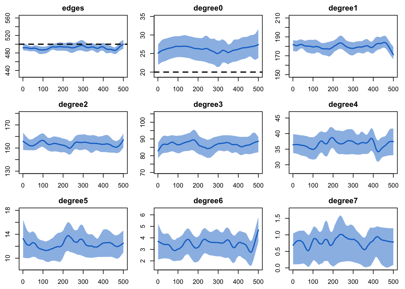

Epidemic Model Parameterization

The epidemic model parameterization for any extension model consists of using the same three input functions as with built-in models.

First we start with the model parameters in param.net. Note that we have two new rates here: ei.rate and ir.rate. These control the transitions from E to I, and then I to R. We have selected these parameter names and input the values here, but note that the same parameters get pulled into the disease progression function above. So in general there must be consistency between the naming of the parameters as inputs and their references in the model functions.

param <- param.net(inf.prob = 0.5, act.rate = 2,
                   ei.rate = 0.01, ir.rate = 0.01)

Next we specify the initial conditions. Here we are specifying that there are 10 infectious individuals at the epidemic outset. If we wanted to initialize the model with persons only in the latent stage, we would need to set disease status as a nodal attribute on the network instead (following the same approach in the Serosorting Tutorial.

init <- init.net(i.num = 10)

Finally, we specify the control settings in control.net. Extension models like this require some significant updates (compared to built-in models) here. First, type is set to NULL in any extension model because we are no longer using EpiModel to pre-select which modules to run; it is an entirely manual process. Second, the new input parameter for the infection.FUN argument is infect; in other words, our new function for our infection module is the one we built above. Note that it is called infect. Third, we are defining a new module, progress.FUN, with an argument that matches the name of our new progression function. We defined a new module, rather than replaced the function of the recovery module, just to show you how to define a new module here. We could have just as easily done it the latter way with the same results. Finally, we are explicitly setting resimulate.network to FALSE; this is the default, so this is not necessary, but it is just to remind you this is a model without network feedback.

source("d4-s9-SEIR-fx.R")
control <- control.net(type = NULL,
                       nsteps = 500,
                       nsims = 1,
                       ncores = 1,
                       infection.FUN = infect,
                       progress.FUN = progress,
                       resimulate.network = FALSE)

In the R scripts that we include with this tutorial, you will see that we have two separate R script files (for the R Markdown build, they all go in this single file). One contains the module functions, and the other contains all the other code to parameterize and run the model. We do this because it allows for easier interaction with the functions in browser mode. I will demonstrate this live next. But in general, placing the functions in a separate file conceptually disentangles the model functionality from the model parameterization. It is critical, however, that you source in the file containing the functions before you run control.net (otherwise, control.net does not know what infect and progress are).

Epidemic Simulation

Finally we are ready to do the epidemic model simulation and analysis. This is done using the same approach as the built-in models. We will start with running one model in the browser mode interactively.

sim <- netsim(est, param, init, control)

And then go back, comment out the browser lines, re-source the functions, and run a full-scale model with 10 simulations.

source("d4-s9-SEIR-fx.R")
control <- control.net(type = NULL,
                       nsteps = 500,
                       nsims = 10,
                       ncores = 5,
                       infection.FUN = infect,
                       progress.FUN = progress,
                       resimulate.network = FALSE)
sim <- netsim(est, param, init, control)

Once the model simulation is complete, we can work with the model object just like a built-in model. Start by printing the output to see what is available.

print(sim)

EpiModel Simulation
=======================
Model class: netsim

Simulation Summary
-----------------------
Model type:
No. simulations: 10
No. time steps: 500
No. NW groups: 1

Fixed Parameters
---------------------------
inf.prob = 0.5
act.rate = 2
ei.rate = 0.01
ir.rate = 0.01
groups = 1

Model Functions
-----------------------
initialize.FUN 
resim_nets.FUN 
infection.FUN 
nwupdate.FUN 
prevalence.FUN 
verbose.FUN 
progress.FUN 

Model Output
-----------------------
Variables: s.num i.num num ei.flow ir.flow e.num r.num 
se.flow
Networks: sim1 ... sim10
Transmissions: sim1 ... sim10

Formation Diagnostics
----------------------- 
        Target Sim Mean Pct Diff Sim SD
edges      500  492.117   -1.577 17.432
degree0     20   25.781   28.905  5.184


Dissolution Diagnostics
----------------------- 
      Target Sim Mean Pct Diff Sim SD
edges   0.04      NaN      NaN     NA

Here is the default plot with all the compartment sizes over time. This includes the new summary statistics we tracked in the disease progression function.

par(mar = c(3, 3, 1, 1), mgp = c(2, 1, 0))
plot(sim)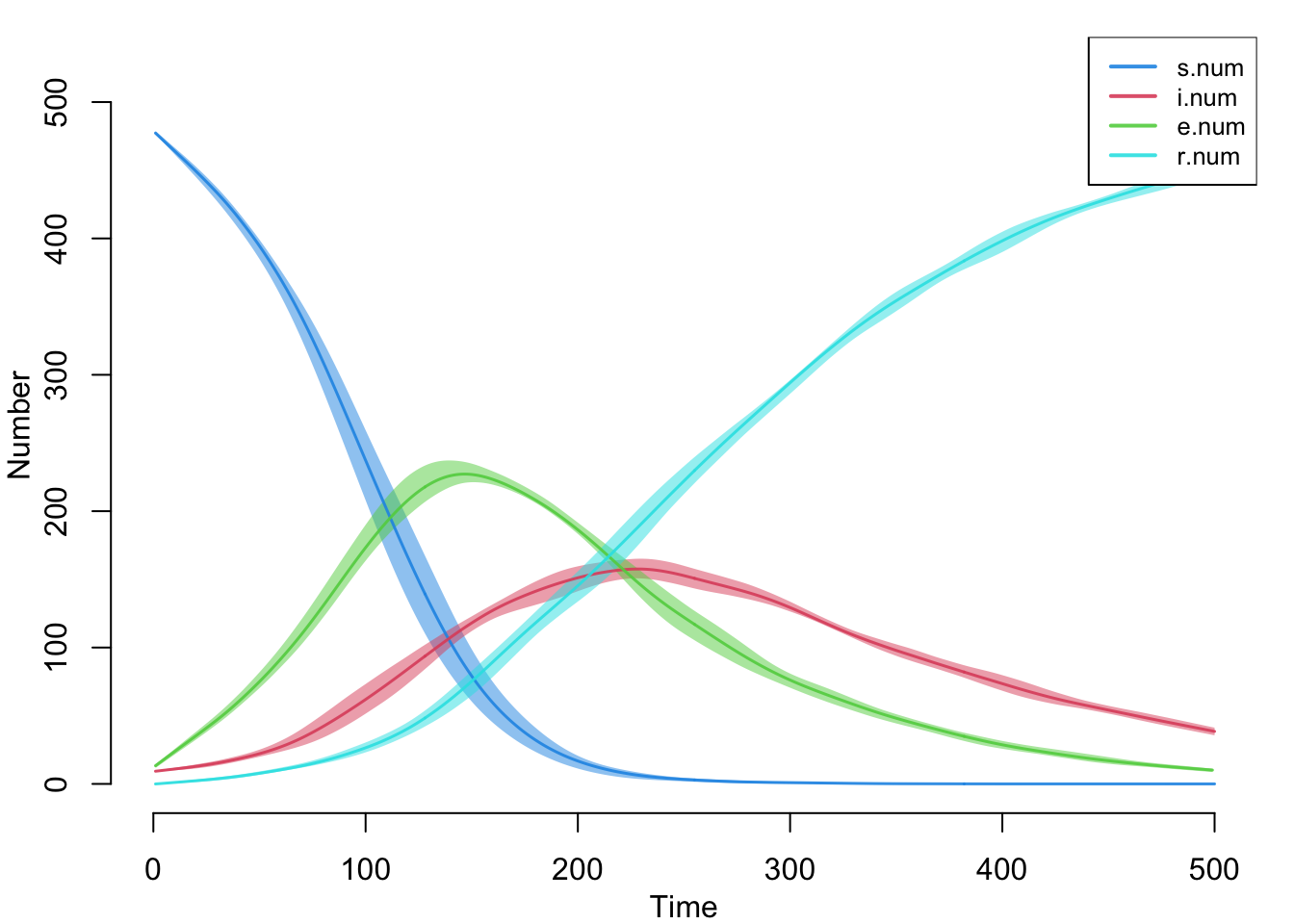

Here are the flow sizes, including the new se.flow incidence tracker that we established in the new infection function.

plot(sim, y = c("se.flow", "ei.flow", "ir.flow"), legend = TRUE)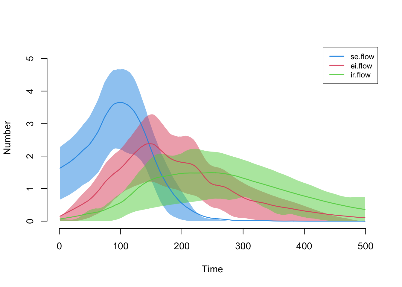

Finally, here is the data frame output from the model, with rows limited to time step 100 across all 10 simulations.

df <- as.data.frame(sim)
df[which(df$time == 100), ]

     sim time s.num i.num num ei.flow ir.flow e.num r.num se.flow
100    1  100   208    77 500       2       0   187    25       3
600    2  100   220    69 500       1       1   187    22       2
1100   3  100   186    72 500       3       3   206    33       3
1600   4  100   297    40 500       2       1   134    26       3
2100   5  100   210    67 500       0       0   188    31       4
2600   6  100   256    55 500       3       1   162    21       6
3100   7  100   308    38 500       1       1   133    17       4
3600   8  100   246    58 500       0       0   166    26       4
4100   9  100   178    81 500       2       0   205    29       7
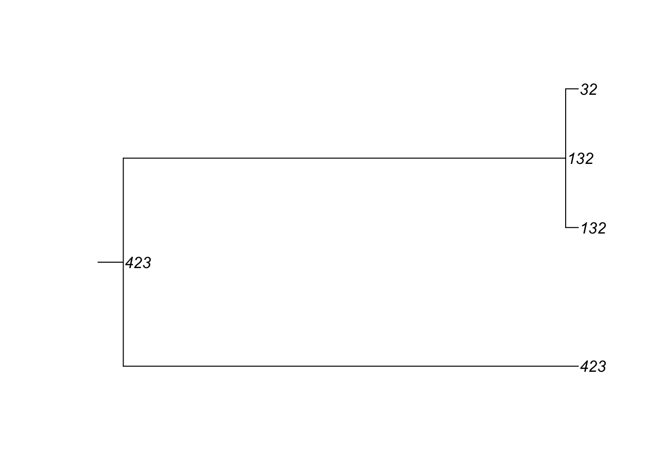
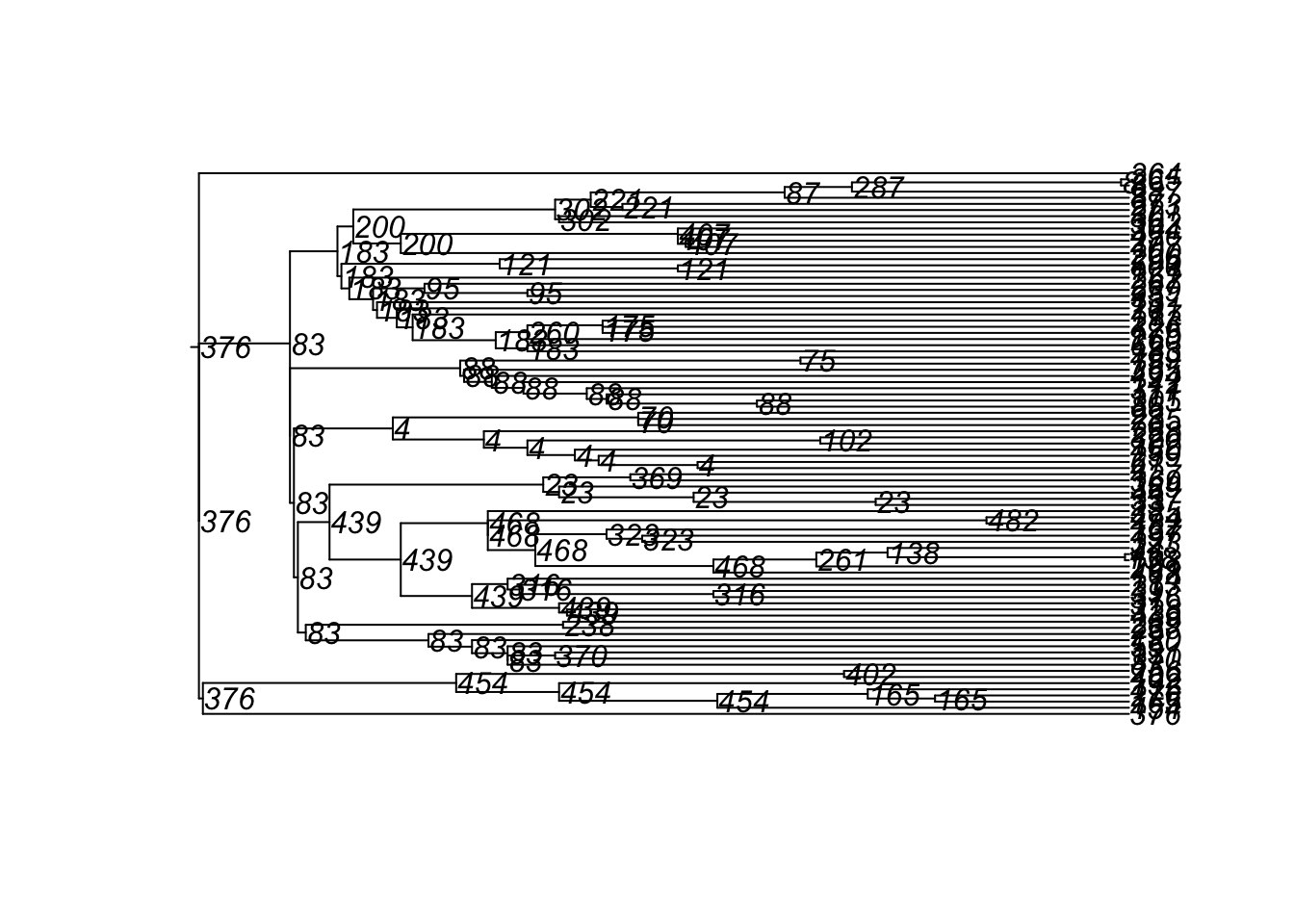
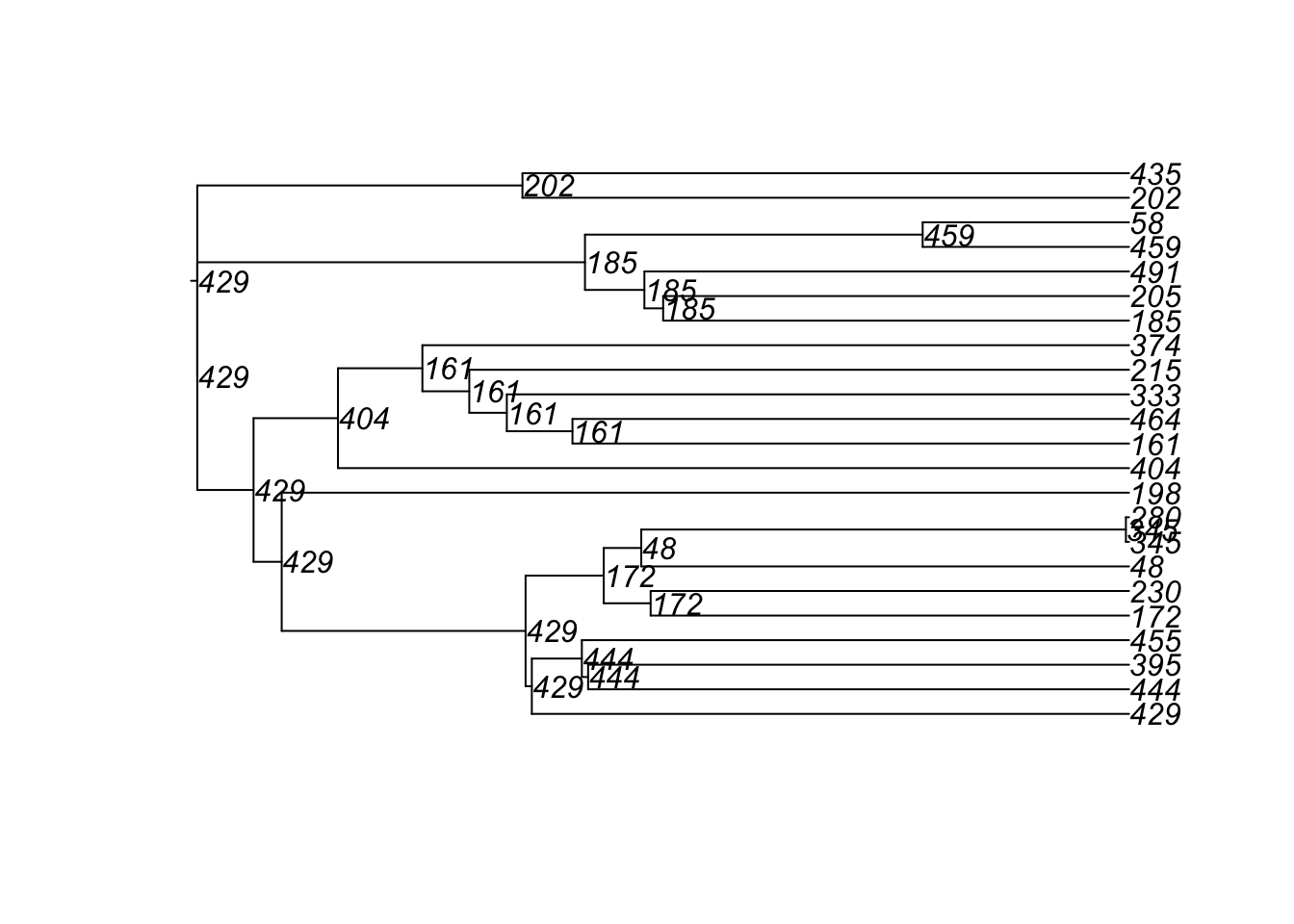
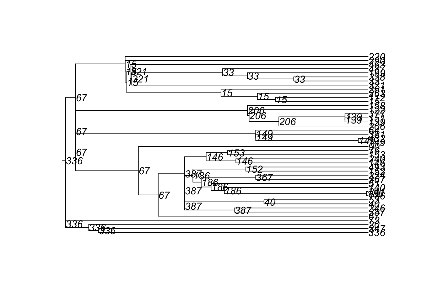
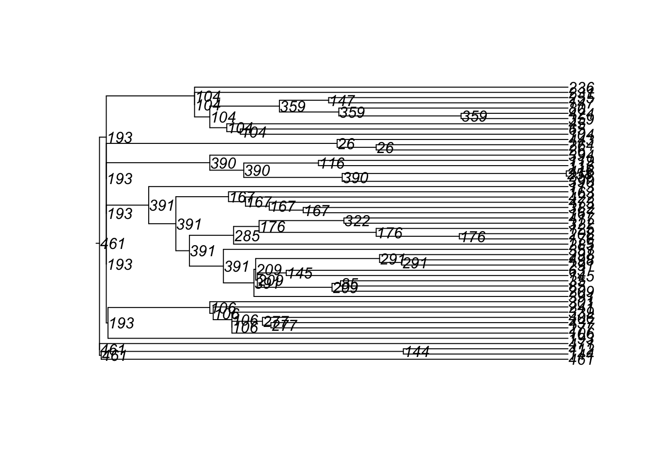
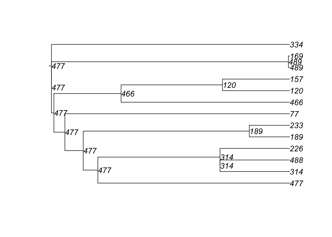
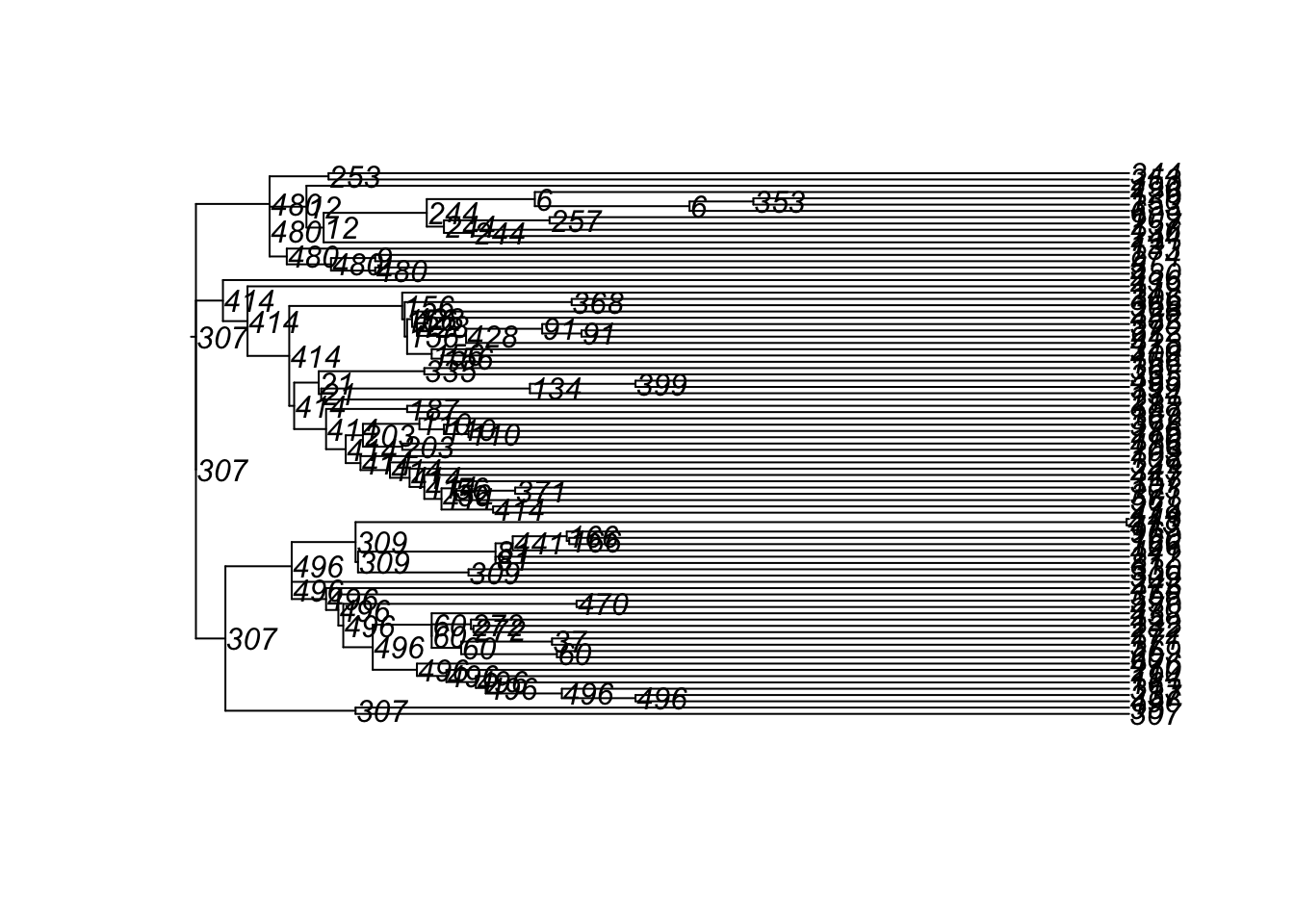
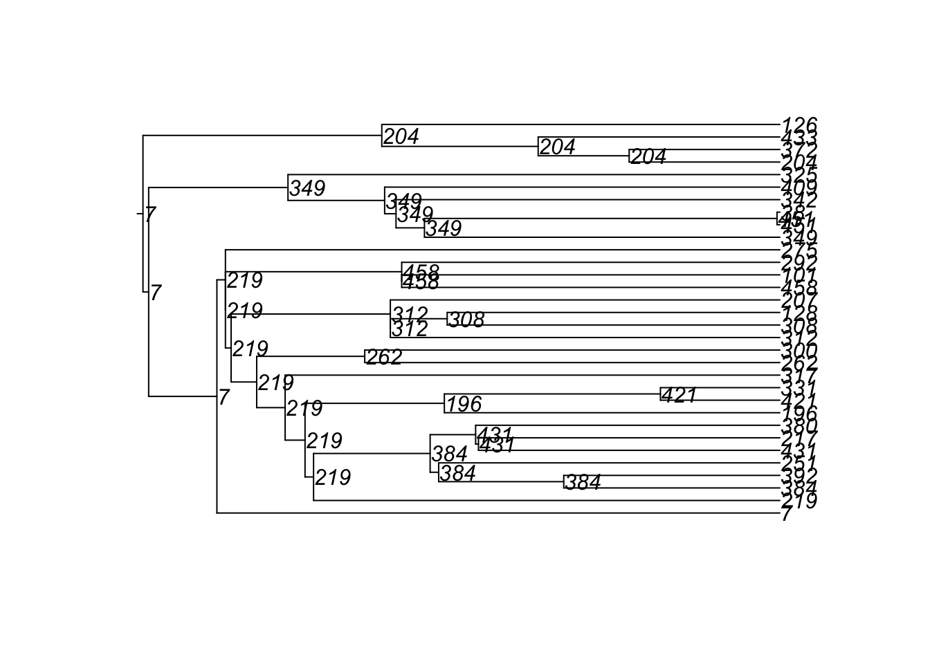
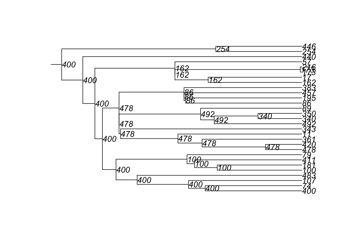
4600  10  100   248    52 500       1       3   167    30       3

And here are the transmission matrices and their phylogram plots (one per infection seed).

tm1 <- get_transmat(sim)
plot(tm1)

found multiple trees, returning a list of 10phylo objects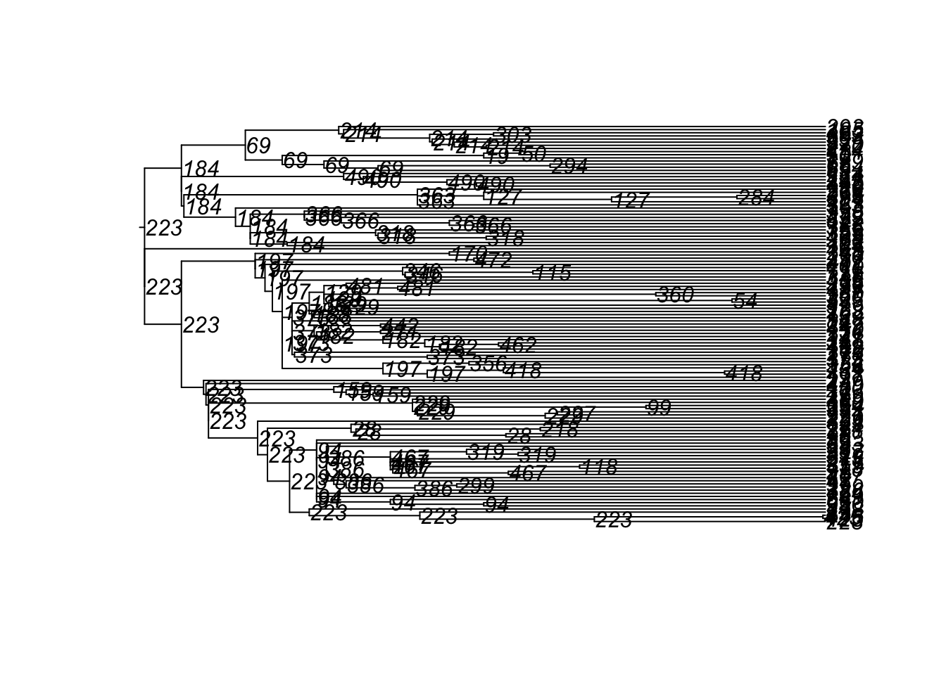

---

Last updated: 2022-07-07 with EpiModel v2.3.0