R Tutorial
R is software for statistical computing. It differs from
many commerical software programs like Stata or SAS in that it is free
and open-source, and that nearly all functionality requires command-line
programming. This brief R tutorial covers the basics of
R functionality to be used in the NME course labs.
Other Resources
This tutorial will not cover everything to know about R.
For a more complete background to learning the language, we recommend
the following:
- Coursera R Programming Course: This online course may be audited so that you may just review the course materials.
- Elementary Statistics with R Introduction
When learning a new programming language, the best method is regular
practice and integration into one’s daily life. Try using R
on a regular basis for data management, analysis, and modeling
tasks.
When stumped, the built-in documentation usually provides a solution.
If not, http://stackoverflow.com/ is a helpful resource; one can
limit search results with an [r] tag in the search box.
Basics
To get started, we will introduce some of the core functionality and
data structures in R. At its core, R is a
fancy calculator with memory.
3*2 [1] 6But it is also a programming language with defined syntax and native
constants like pi.
# Comments are embedded in code with a #
4*pi
[1] 12.56637Separate commands need to be put on separate lines, unless a
; is used.
letters [1] "a" "b" "c" "d" "e" "f" "g" "h" "i" "j" "k" "l" "m" "n" "o" "p" "q" "r" "s"
[20] "t" "u" "v" "w" "x" "y" "z"LETTERS [1] "A" "B" "C" "D" "E" "F" "G" "H" "I" "J" "K" "L" "M" "N" "O" "P" "Q" "R" "S"
[20] "T" "U" "V" "W" "X" "Y" "Z"R contains many arithmetical functions.
round(4.2)[1] 4ceiling(4.2)[1] 5floor(4.2)[1] 4Packages
R is built on a foundation of functions installed with
the base R program. A strength of R is the
extension of this software through easily accessible built in packages
contributed by users. EpiModel, ergm, and
network are examples of packages. Most add-on packages are
available through CRAN, the central repository for R. You
can install any package from CRAN by simply typing:
install.packages("packagename")This will typically install not only the package but all the related packages needed. Once a package is installed, it may be loaded for use by typing:
library("packagename")Help and Documentation
Help files are accessed through the console in either of the following ways.
?mean
help("mean")
A help index is available for all contributed packages like
EpiModel by typing:
help(package = "EpiModel")Many packages have built-in documentation (called vignettes) that are
accessible for the network package, for example, by
typing:
browseVignettes("network")Objects
Nearly all R programming is “object-oriented”. To assign a value to
an object, use <-.
a <- 3 To evaluate an object, type its name in the console window.
a[1] 3Once an object is stored, it may be called for further operations.
a*2[1] 6b <- a/2
b[1] 1.5To test the value of an object, use ==.
a == 3[1] TRUEa^2 == 8[1] FALSETo test inequality, use !=.
a != 3[1] FALSEa != 4[1] TRUETo see the list of objects in the current environment:
ls()[1] "a" "b"Vectors
To create a vector of one element repeated many times, use
rep (for repeat)
rep(4, 10) [1] 4 4 4 4 4 4 4 4 4 4To create a vector with different elements, use c (for
combine).
d <- c(4, 3, 1, 7)
d
[1] 4 3 1 7These can be combined arbitrarily to create a chained vector.
c(rep(9, 5), 6, 1, rep(5, 9)) [1] 9 9 9 9 9 6 1 5 5 5 5 5 5 5 5 5Colon notation gives you a vector of sequential integers.
1:10 [1] 1 2 3 4 5 6 7 8 9 10Square brackets pull out elements from a vector.
d[2] [1] 3d[2:3][1] 3 1Negative in a bracket means “eveything but”.
d[-2][1] 4 1 7Empty Vectors
If you want to make a vector but leave it empty for the moment (useful to time-series simulations), there are several options. The following is simplest when you do not know the size of the vector in advance.
f <- vector()
flogical(0)If you do know the vector size, it is preferable to create a
non-empty vector filled with an arbitrary value that will never be used
for a true value. Here, we create a vector with a length of 10, which
for the moment are filled with a missing data value NA.
Note that when we put an assignment operation in parentheses,
R will print the outcome of that assignment to the console.
Spaces around any operations are acceptable, but it is recommended that
you use a clear and consistent coding type (for example: http://adv-r.had.co.nz/Style.html) so that others can
easily read your work.
( g <- rep(NA, 10) ) [1] NA NA NA NA NA NA NA NA NA NANext we fill in the vector with values 0 and 1. The elements 1, 2, 3,
4, 6, and 9 are given the value of 1. Next, we use the
is.na function to find which elements in the vector are
equal to NA, and then assign the value of 0 to those
elements.
g[c(1:4, 6, 9)] <- 1
g[is.na(g)] <- 0
g
[1] 1 1 1 1 0 1 0 0 1 0Evaluating Vectors
Evaluation can be done for vectors too.
g == 1 [1] TRUE TRUE TRUE TRUE FALSE TRUE FALSE FALSE TRUE FALSETo get global summaries of vector evaluations, use the
any and all functions.
any(g == 1)[1] TRUEall(g == 1)[1] FALSETo return the positions of the elements that fulfill a criterion, use
which.
which(g == 1) [1] 1 2 3 4 6 9To see the length of a vector, use the length function.
length(g)[1] 10Basic arithmetic functions for vectors are possible.
mean(g)[1] 0.6Missing Data
For missing data: use NA.
i <- c(3, NA, 1) Operations on NA will return NA.
i*2 [1] 6 NA 2i == 1[1] FALSE NA TRUEMany built-in functions will not simply ignore NA
values, but base their default output on them. The mean or sum of any
vector with an NA will always be NA.
mean(i)[1] NAsum(i)[1] NAHowever, there is often an option to override this default, thereby calculating the statistics by dropping those missing values.
mean(i, na.rm = TRUE)[1] 2sum(i, na.rm = TRUE)[1] 4Set Theory
R includes several set theory functions to evaluate vectors.
a <- 1:10
b <- 5:15
union(a,b)
[1] 1 2 3 4 5 6 7 8 9 10 11 12 13 14 15intersect(a,b)[1] 5 6 7 8 9 10setdiff(a,b)[1] 1 2 3 4setdiff(b,a)[1] 11 12 13 14 15The %in% function is a general way to evaluate vectors
of arbitrary length to see if there are any matches between the
vectors.
a <- 1:3
b <- 2:3
a %in% b
[1] FALSE TRUE TRUEIt may be used to check whether an object matches at least one element of a vector.
type <- "SIR"
type %in% c("SIR", "SIS")
[1] TRUETo test an inequality of a match, the ! must be on the
outside of the entire evaluation:
!(type %in% c("SIR", "SIS"))[1] FALSEMatrices and Arrays
Vectors may be combined into matrixes or arrays of arbitrary
complexity. Note the use of the paste function to make
character vectors to create row and column names.
a <- 1:25
m <- matrix(a, nrow = 5, ncol = 5)
rownames(m) <- paste("row", 1:5, sep="")
colnames(m) <- paste("col", 1:5, sep="")
m
col1 col2 col3 col4 col5
row1 1 6 11 16 21
row2 2 7 12 17 22
row3 3 8 13 18 23
row4 4 9 14 19 24
row5 5 10 15 20 25Here is a three dimensional array. We create a second vector by
multipying each element of m by 2.
n <- m*2
( a <- array(c(m, n), dim=c(5, 5, 2)) )
, , 1
[,1] [,2] [,3] [,4] [,5]
[1,] 1 6 11 16 21
[2,] 2 7 12 17 22
[3,] 3 8 13 18 23
[4,] 4 9 14 19 24
[5,] 5 10 15 20 25
, , 2
[,1] [,2] [,3] [,4] [,5]
[1,] 2 12 22 32 42
[2,] 4 14 24 34 44
[3,] 6 16 26 36 46
[4,] 8 18 28 38 48
[5,] 10 20 30 40 50Note R includes complex matrix albegra functions that we
will not cover here (for example see help("%*%") for matrix
multiplication).
Reference Values
Rows, columns, and cells for matrices may be accessed using the bracket notation. Pull out rows by position:
m[1:2, ] col1 col2 col3 col4 col5
row1 1 6 11 16 21
row2 2 7 12 17 22Pull out columns by position:
m[, 1:2] col1 col2
row1 1 6
row2 2 7
row3 3 8
row4 4 9
row5 5 10Pull out a specific cell:
m[3,3][1] 13Change the value of that cell:
m[3,3] <- 100
m
col1 col2 col3 col4 col5
row1 1 6 11 16 21
row2 2 7 12 17 22
row3 3 8 100 18 23
row4 4 9 14 19 24
row5 5 10 15 20 25Note that when pulling single rows or columns, the matrix will be converted to a vector.
m[, 1]row1 row2 row3 row4 row5
1 2 3 4 5 Often this is necessary to retain the matrix organization. This is possible by:
m[ , 1, drop = FALSE] col1
row1 1
row2 2
row3 3
row4 4
row5 5Arrays can be refernced by position through more commas for each added dimension. This will output the first level of the third dimension.
a[, , 1] [,1] [,2] [,3] [,4] [,5]
[1,] 1 6 11 16 21
[2,] 2 7 12 17 22
[3,] 3 8 13 18 23
[4,] 4 9 14 19 24
[5,] 5 10 15 20 25This will output the second column across both levels of the third dimension.
a[, 2, ] [,1] [,2]
[1,] 6 12
[2,] 7 14
[3,] 8 16
[4,] 9 18
[5,] 10 20Again, as above, to keep that in a three-dimensional array class, use the same syntax as above.
a[, 2, , drop = FALSE], , 1
[,1]
[1,] 6
[2,] 7
[3,] 8
[4,] 9
[5,] 10
, , 2
[,1]
[1,] 12
[2,] 14
[3,] 16
[4,] 18
[5,] 20Adding to a Matrix
Use rbind to add rows to a matrix and cbind
to add columns. First, we use the seq function to generate
a vector of length 5, that starts with the value of 6.
m <- rbind(m, seq(6, 26, 5))
m
col1 col2 col3 col4 col5
row1 1 6 11 16 21
row2 2 7 12 17 22
row3 3 8 100 18 23
row4 4 9 14 19 24
row5 5 10 15 20 25
6 11 16 21 26Next, we use the max function to find the maximum value
of m, a generate a vector of sequential integers that
starts with one higher than that max and ends with 6 higher than that
max.
m <- cbind(m, (max(m) + 1):(max(m) + 6))
m
col1 col2 col3 col4 col5
row1 1 6 11 16 21 101
row2 2 7 12 17 22 102
row3 3 8 100 18 23 103
row4 4 9 14 19 24 104
row5 5 10 15 20 25 105
6 11 16 21 26 106Data Frames
Matrices can only store elements of the same type (e.g., only numeric
or only character), but as this is a limitation for storing datasets,
the data.frame object class may be used. The main
restriction with data frames is that each column (variable) must have
the same length (same number of observations).
id <- 1:10
sex <- c(rep("Female", 5),rep("Male", 5))
( h <- data.frame(id, sex) )
id sex
1 1 Female
2 2 Female
3 3 Female
4 4 Female
5 5 Female
6 6 Male
7 7 Male
8 8 Male
9 9 Male
10 10 MaleData frames may be accessed using the same bracket notation as above if you want to operate on them by position. But they may also be referenced by column name:
h$sex [1] "Female" "Female" "Female" "Female" "Female" "Male" "Male" "Male"
[9] "Male" "Male" Subset the data frame by variable values. Inside the bracket is a logical evaluation statement to test when each row satisfied two conditions jointly.
h[h$sex == "Female" & h$id < 5, ] id sex
1 1 Female
2 2 Female
3 3 Female
4 4 FemaleObtain the dimensions of a data frame (rows first, columns second).
dim(h)[1] 10 2The outputs of functions are themselves objects, which can be evaluated and operated on in turn.
nrows.h <- nrow(h)
ncols.h <- ncol(h)
c(nrows.h, ncols.h) == dim(h)
[1] TRUE TRUETo obtain general “meta-data” on a data frame (or any R
object), use:
str(h)'data.frame': 10 obs. of 2 variables:
$ id : int 1 2 3 4 5 6 7 8 9 10
$ sex: chr "Female" "Female" "Female" "Female" ...Conditional Logic
Conditional logic is heavily used in R to evaluate
vectors and calculate object values based on those conditions.
If Statements
If statments evaluate the value of a single element of a vector (i.e., a scalar); if the condition is true, then the code following the conditional evaluation will be run, or otherwise, skipped. Note the syntax that the evaluation condition must go in parentheses.
a <- 3
if (a > 5) j <- 99
if (a < 5) j <- 77
j
[1] 77If/Else Statements
If/Else Statements enforce a counterfactual to the first conditional evaluation. If the conditional is false, then the else alternative must be true, and the code is evaluated. Note the use of brackets here to put the assignment operation on a following line. This is generally the best style choice as it makes the “then” part unambiguous.
if (j == 77) {
  k <- j+1
} else {
  k <- j-1
}
k
[1] 78The ifelse Function for Vectors
As noted, the statements above only work for single elements to be
evaluated. R includes the ifelse function to
evaluate multiple length vectors such as the following. Note the use of
sample to generate a random vector choosing equally among
three races with replacement. The ifelse function then
evaluates the race vector, and if that condition is true,
sets the new variable white.race to be TRUE,
otherwise to be FALSE. Finally we store the results in a
data frame.
race <- sample(c("Black", "White", "Asian"), size = 10, replace = TRUE)
white.race <- ifelse(race == "White", TRUE, FALSE)
( df <- data.frame(race, white.race) )
race white.race
1 Asian FALSE
2 White TRUE
3 Black FALSE
4 White TRUE
5 White TRUE
6 White TRUE
7 White TRUE
8 White TRUE
9 Asian FALSE
10 Asian FALSELoops
Loops in R are the core method to simulate epidemic
models because the values at any time step depend on the stochastic
realizations of the previous step: an iterative process is needed.
For Loops
In the following, we recreate a proportional growth model in which
new infections are a function of the prevalence at the prior time step
and a fixed growth rate. In the loop, we create an iterator,
i, which runs from time 2 to the number of time steps (10)
in sequential integers. We initialize the vector prevalence
to save the output, and start with its initial value of the
initial.infected. Then we update the prevalence vector for
each time step i by calling the value of that vector at the
prior time step and performing the basic calculation.
initial.infected <- 20
time.steps <- 10
growth.rate <- 0.2

prevalence <- initial.infected
for (i in 2:time.steps) {
  prevalence[i] <- prevalence[i-1] + prevalence[i-1]*growth.rate
}
prevalence
[1] 20.00000 24.00000 28.80000 34.56000 41.47200 49.76640 59.71968
[8] 71.66362 85.99634 103.19561While Loops
While loops are a useful, but less common way to update vectors based on conditions. Intead of some interation in time, while loops require that a condition be satisfied to evaluate their contents. Below we track prevalence now without history as a single element vector; the loop will continue to run as long as prevalence is below 50. Note that the final value of prevalence is above 50 because it does not evaluate prevalence until after the previous iteration is run.
prevalence <- initial.infected
while (prevalence < 50) {
  prevalence <- prevalence + prevalence*growth.rate
}
prevalence
[1] 59.71968Functions
All of R is functions. At their basic, functions take an
input, run calculations, and supply an output.
A Basic Function
Below, we define a function f, which takes as input two
arguments, x and y, and returns their
product.
f <- function(x, y) x*y
f(3, 5)
[1] 15Because R is an interpreted rather than compiled
language (like C or C++), there is no
guarantee that any function will work. Robust functions, like those in
R packages, have a set of input checks to prevent errors
like this. The problem here, of course, if that * (itself a
function!) expects a numeric input but we have supplied a character
vector.
f("Male", "Female")Error Checking and Return
When building new functions, we could write in an error check to make
sure problems like these are identified early and clearly. Below, we set
our own error message (that is not much more helpful than the error
message supplied by *) early in the function. If either
x or y in the function are not numeric, then
the function will stop and print the error message. Otherwise, they will
be evaluated and returned. Note that an explicit return call must be
used in functions if any object assignment is conducted within the
function.
f <- function(x, y) {
  if (!is.numeric(x) | !is.numeric(y)) {
    stop("x and y must be numeric!!")
  }
  out <- x*y
  return(out)
}
Stochastic Growth
As an extended example, we build on our proportional growth model
above, and add elements of stochasticity into the model. If we specify
that stochastic=TRUE when we call the function, it will add
a random draw from a normal distribution to the growth rate. Here we
have incorporated many elements of the tutorial: functions, for loops,
conditional logic, and operations on vectors!
pg.model <- function(initial.infected, time.steps,
                     growth.rate, stochastic) {
  prevalence <- initial.infected
  for (i in 2:time.steps) {
    if (stochastic == TRUE) {
      prevalence[i] <- prevalence[i-1] +
                       prevalence[i-1]*(growth.rate +
                                        rnorm(1, mean = 0.1, sd = 0.01))
    } else {
      prevalence[i] <- prevalence[i-1] +
                       prevalence[i-1]*growth.rate
    }
  }
  return(prevalence)
}
We run the model twice with the same parameter values but once as deterministic and once as stochastic. Note that it is not necessary to specify the argument names when calling a function, as long as the order of argument inputs is correct.
pg.model(initial.infected = 20, time.steps = 10,
         growth.rate = 0.2, stochastic = FALSE)
[1] 20.00000 24.00000 28.80000 34.56000 41.47200 49.76640 59.71968
[8] 71.66362 85.99634 103.19561pg.model(20, 10, 0.2, TRUE) [1] 20.00000 25.80052 33.94291 44.87257 57.65415 75.20996 98.39125
[8] 127.31031 163.75326 211.23476Statistical Distributions
In stochastic epidemic modeling, it is necessary to draw from
statistical distributions to determine, for example, the number of
births that will occur in a time step given a population size and a
birth rate. For discrete events, we most often use the Poisson and
binomial distribution functions in R. The r
prefix on each distribution generates one or several random draws from
that distribution with the parameters set in the function.
Normal Distribution
round(rnorm(n = 5, mean = 100, sd = 10), 1)[1] 116.2 95.0 99.3 113.0 93.9Poisson Distribution
popsize <- 1000
birthrate <- 0.01
rpois(n = 5, lambda = popsize*birthrate)
[1] 12 19 17 6 17Binomial Distribution
transmission.rate <- 0.5
rbinom(n = 10, size = 1, prob = transmission.rate)
[1] 0 0 0 0 0 0 1 1 0 1Uniform Distribution
runif(n = 10) <= transmission.rate [1] FALSE TRUE TRUE FALSE FALSE FALSE TRUE FALSE FALSE TRUEPlotting
R excels at data visualization, but often some work is
involved in tweaking the graphical parameters. Plots can be as
arbitrarily complex as needed. Let’s set a three variable plot (perhaps,
height by weight by age). We will sample values for x,
y, and z from three different
distributions.
n <- 25
x <- sort(sample(20:220, n))
y <- 10 + 2*x + rnorm(n, 0, 10)
z <- rpois(n, 10)
The build in plot function defaults will produce a quick output.
plot(x, y, cex = z/4)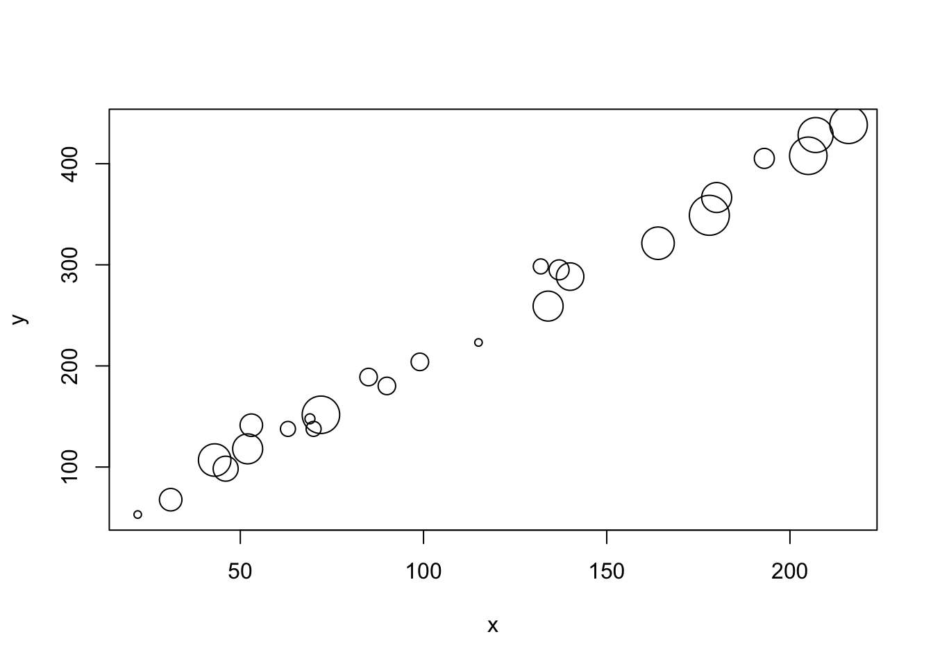
But it is possible to make many graphical choices for beautiful output for presentations and publications. To see what’s going on here, see the help documentation for each of these functions.
tcol <- adjustcolor("steelblue", alpha.f = 0.5)
plot(x, y, cex = z/4, pch = 21, col = "black", bg = tcol,
     lwd = 1.2, axes = FALSE, ylim = c(0, 500), xlim = c(0, 250),
     yaxs = "r", xaxs = "r")
axis(2, seq(0, 500, 100), col = "white", las = 2,
     cex.axis = 0.9, mgp = c(2, 0.5, 0))
axis(1, seq(0, 250, 50), cex.axis = 0.9, mgp = c(2, 0.5, 0))
abline(h = seq(100, 500, 100), col = adjustcolor("black", alpha.f = 0.35))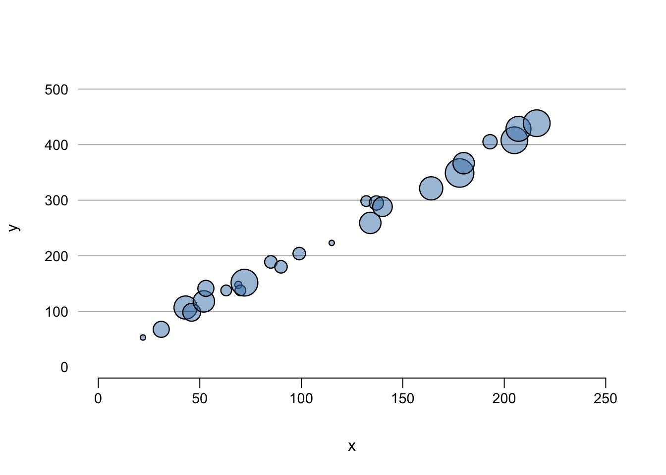
Last updated: 2022-07-07